Video spatial generation is the task of synthesizing a temporally coherent image sequence (a video clip) from a high-level prompt together with optional spatial, temporal, and other conditioning signals. It has advanced substantially in recent years, evolving from early generative adversarial network (GAN)-based approaches [1646] through autoregressive token models to the diffusion- and diffusion-transformer-based systems that now dominate the field [1988, 1989, 1990, 1991]. This rapid progress has stimulated a wide range of downstream tasks, extending beyond basic text-to-video generation to encompass fine-grained control mechanisms (spatial, e.g., , image, pose, depth, landmark, sketch, and bounding box; temporal, e.g., , optical flow, trajectory, camera, and motion; and other conditional controls, e.g., , style, audio, bird’s-eye view) as well as sophisticated video editing capabilities.
Within the arc of §8, video spatial generation is the temporal extension of the priors built in the preceding two sections. Whereas §8.1 learned a 2D semantic-to-pixel prior on a single image plane and §8.2 lifted that prior into a static volumetric representation, this section adds the time axis: the model must place matter and appearance correctly and make them evolve plausibly as the camera or the scene itself moves through time. Appearance, geometry, and dynamics must now be jointly consistent: a generated clip is judged not only frame by frame but on object permanence, motion plausibility, and multi-view coherence under camera motion, which makes video the natural substrate for the dynamic world models and simulators that consume spatial structure downstream.
Formally, we cast every system in this section as a conditional spatio-temporal sampler that extends the latent-generator framework of §8.1.1. Let be the space of -frame clips and a compressed spatio-temporal latent space supplied by a video autoencoder that extends the image autoencoder of Eq. (8.1) along the time axis. Writing for the text encoder of Eq. (8.2) and for a generic encoder of an auxiliary control signal , the core learning problem is to train
| (8.41) |
so that the decoded clip is photorealistic, temporally coherent, and faithful to both the prompt and the control . Two limiting cases anchor the framework: with no auxiliary control () Eq. (8.41) reduces to text-to-video generation, and with a single frame () it recovers the image generator of Eq. (8.2) exactly, so video spatial generation is precisely the image prior of §8.1 unrolled in time and equipped with a richer conditioning interface.
The subsections are organized by the axis of control each introduces into Eq. (8.41). Text-to-video generation (§8.3.1) is the base case without auxiliary control; spatial control (§8.3.2) adds a per-frame scaffold such as a pose or depth sequence; temporal control (§8.3.3) adds a motion or camera signal that governs dynamics rather than appearance; §8.3.4 covers the remaining modalities and the frameworks that fuse several at once; and video editing (§8.3.5) modifies an existing clip, lifting the 2D editing of §8.1.3 into time. §8.3.6 compares the five and discusses the challenges they share.
8.3.1Text-to-Video Generation#
Text-to-video (T2V) generation [1991, 1988, 1989, 1990] synthesizes photorealistic, temporally coherent video from a natural-language description. It extends text-to-image (T2I) synthesis along time, so the model must produce plausible motion and state transitions as well as high-fidelity frames, and it does so with no explicit spatial scaffold: object permanence, motion plausibility, and view coherence under camera motion cannot be supplied from outside but must emerge from the generator itself. That is why the unconditional T2V model is the substrate on which the explicit control axes of §8.3.2–§8.3.5 are built. Its architecture has followed the image case, from generative adversarial networks (GANs) through autoregressive models to the diffusion models that dominate today, with progress driven as much by data as by architecture [1992, 1993].
8.3.1.1Task Definition#
8.3.1.2Methodology#
The three paradigms factorize the clip distribution adversarially, causally over discrete tokens, or by iterative spatio-temporal denoising, and each changes its image counterpart of §8.1.1 in one structural respect; Figure 8.13 contrasts how each handles the temporal dimension.
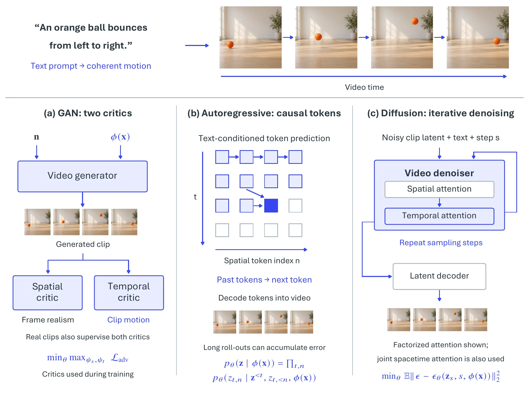
Generative Adversarial Networks (GANs). The first T2V systems extended the image GANs of §8.1.1.2 to clips. The video-specific change is in the discriminator: rather than scoring a single image, it must judge both per-frame realism and the plausibility of motion across the sequence, which is naturally realized as a two-critic objective
| (8.43) |
where is the decoded clip, the spatial critic scores individual frames, and the temporal critic scores motion coherence over the clip, the term absent from the single-discriminator image objective of Eq. (8.3). TGAN [1994] and TGAN-v2 [1995] used a temporal generator to produce latent motion vectors from which an image generator rendered frames; MoCoGAN [1996] and MoCoGAN-HD [1997] disentangled content from motion, generating the motion code recurrently; DVD-GAN [1998] instantiated Eq. (8.43) directly with separate spatial and temporal discriminators; and DIGAN [1999] used implicit neural representations for longer sequences. Even with architectures such as StyleGAN-V [2000], GANs suffered from flicker, training instability, and mode collapse, which limited the diversity of their motion and pushed the field toward other paradigms.
Autoregressive Models. Autoregressive (AR) models recast T2V as the sequential prediction of §8.1.1.2, tokenizing a clip with a 3D Vector Quantized Variational Autoencoder (3D VQ-VAE) and predicting each token from its predecessors with a large transformer. The video-specific change is the order of the factorization: where the image model of Eq. (8.4) runs over the spatial tokens of a single frame, the video model factorizes over space and time,
| (8.44) |
so that each frame is conditioned on all previously generated frames . This inter-frame causal dependency is the source of both the paradigm’s strength (global temporal coherence) and its characteristic failure, the accumulation of per-step error over long roll-outs. VideoGPT [27] demonstrated the approach for unconditional generation, NÜWA [2001] and CogVideo [1989] adapted it to text-to-video synthesis, and TATS [2002] addressed quality degradation in long sequences. The paradigm has since resurged in large multimodal backbones: Emu3 [2003] generates video inside a language-model backbone by treating frames as discrete visual tokens, and CausVid [2004] and MAGI-1 [2005] scale to long-form generation with autoregressive diffusion transformers. Sequential decoding nevertheless remains expensive and prone to the error accumulation that Eq. (8.44) makes explicit.
Diffusion Models. Diffusion models, which now dominate T2V, lift the latent-denoising objective of §8.1.1.2 from a single image to the clip latent . The forward and reverse processes are those of Eq. (8.5); the video-specific change is that the denoiser operates on a spatio-temporal tensor and is trained to predict the noise added to the whole clip at sampling step ,
| (8.45) |
where models dependencies across both space and time, and is distinct from the frame index . One widely used design factorizes attention into spatial attention within each frame and temporal attention across frames, as illustrated in Figure 8.13(c); other architectures use joint spacetime attention. VDM [2006] applied the idea in pixel space with a 3D U-Net; the breakthrough was moving diffusion into the compressed latent space of a video-specific autoencoder, as in VideoLDM [2007], LVDM [2008], and the open-source Stable Video Diffusion (SVD) [1873], which cut training and inference cost enough to make high-resolution generation practical.
A second recipe adapts pretrained T2I models. Imagen Video [2009] and Make-A-Video [2010] freeze a T2I model and insert trainable temporal modules (e.g., , temporal attention layers or 1D convolutions) between its spatial layers, which are then trained on video to learn motion while the image prior is inherited intact. VideoCrafter [2011, 2012] and LaVie [2013] built high-quality generators on this recipe, Tune-A-Video [2014] adapted it to one-shot tuning on a single clip, and AnimateDiff [2015] turned the temporal modules into plug-and-play motion modules that animate personalized T2I models without further fine-tuning.
Diffusion Transformers (DiTs) have since replaced the U-Net backbone, operating on “spacetime patches” (unified tokens representing blocks of video) and scaling well. Sora [1991] demonstrated long-duration (up to one minute), high-resolution clips and presented the approach as a step toward world simulation, and a wave of DiT models followed, including Open-Sora [2016], LATTE [2017], CogVideoX [2018], StepVideo [2019], Movie Gen [1988], Wan [1990], and Veo [2020]. Large open DiT foundation models have substantially narrowed the gap to proprietary systems. HunyuanVideo [2021], at B parameters the largest open T2V model at release, couples a “dual-stream-to-single-stream” full-attention DiT (text and video tokens processed in separate streams before fusion) with a multimodal-LLM text encoder and a 3D causal VAE, and reports human-evaluated quality competitive with leading closed systems. Mochi 1 [2022] introduces an asymmetric DiT (AsymmDiT) that allocates most capacity to the visual stream, and LTX-Video [2023] uses a high-compression video VAE to run latent video diffusion in near real time. NVIDIA’s Cosmos [156] reframes the video generator as a world-foundation model for “Physical AI”, trained so that embodied and robotics systems can use it as a learned simulator, which ties video generation to the world models of §8.6. Across these shifts the T2V trajectory has trailed the T2I trajectory of §8.1.1 by roughly a year, each image paradigm being inflated along the time axis once it matured.
8.3.1.3Benchmarks#
Video adds a requirement at every level of evaluation: corpora must pair clips with captions at scale, suites must stratify by temporal phenomena (motion, object permanence, dynamic degree), and metrics must measure cross-frame coherence as well as per-frame quality.
Training Corpora. Caption–clip scale has been the principal driver of T2V quality, and high-quality paired video–text data is far scarcer than image–text data. Early work repurposed action-recognition corpora such as UCF-101 [902] and Kinetics [239], which supply short, class-labeled clips but no captions. WebVid-10M [2024], the first web-scale captioned corpus, underpinned most 2022–2023 systems despite noisy alt-text captions and watermarks; later corpora raised caption density and clip length, with Panda-70M [1992] captioned automatically by cross-modality teachers, MiraData [1993] targeting long clips with dense structured captions, and Koala-36M [2025] explicitly optimizing the consistency between caption and content, the property that most directly limits a generator’s controllability. Table 8.7 gives their scale.
| Corpus | Year | Scale | Annotation / Notes |
| UCF-101 [902] | 2012 | 13,320 clips | 101 action classes; labels, no captions |
| Kinetics [239] | 2017 | 650K clips | Action classes; labels, no captions |
| WebVid-10M [2024] | 2021 | 10M clip–text pairs | Web alt-text captions; noisy, watermarked |
| Panda-70M [1992] | 2024 | 70M clip–text pairs | Auto-captioned by cross-modality teachers |
| MiraData [1993] | 2024 | 330K clips | Long-duration; dense structured captions |
| Koala-36M [2025] | 2025 | 36M clip–text pairs | Fine-grained structured captions; condition–content consistency |
Evaluation Benchmark Suites. Classical T2V evaluation reported zero-shot distributional scores on the held-out splits of UCF-101 and MSR-VTT [2026], which probe frame quality and coarse text relevance but say nothing about temporal or compositional faithfulness. Recent suites are purpose-built: VBench [1951] decomposes quality into fine-grained dimensions (subject and background consistency, motion smoothness, dynamic degree, temporal flicker, per-frame aesthetic and imaging quality), each with an automatic protocol validated against human preference; EvalCrafter [2027] aggregates objective metrics over prompts derived from real-world usage; and T2V-CompBench [2028] targets compositional faithfulness over time (attribute binding, spatial relations, motion binding, interactions), the temporal analogue of the T2I-CompBench probe of §8.1.1. Table 8.8 lists them.
| Suite | Year | Evaluation Axis | Scoring |
| UCF-101 / MSR-VTT [902, 2026] | 2012–16 | Frame quality coarse text relevance (MSR-VTT: 10K captioned clips) | Zero-shot FVD / IS / CLIPSIM |
| VBench [1951] | 2024 | 16 dimensions (consistency, motion, dynamics, flicker, quality) | Per-dimension automatic, human-validated |
| EvalCrafter [2027] | 2024 | 17 objective metrics over 700 structured prompts | Aggregated automatic, fitted to human opinion |
| T2V-CompBench [2028] | 2024 | Compositional: attribute/motion binding, relations, interactions | MLLM- / detector-based |
Evaluation Metrics. The metric that defines video evaluation is the Fréchet Video Distance (FVD) [1950], the spatio-temporal analogue of FID: it compares distributions of features extracted from generated and real clips by a pretrained video backbone (I3D), and is therefore sensitive to motion realism in a way that per-frame FID [1681] and Inception Score are not. Text–clip alignment is measured by CLIPSIM, the per-frame CLIPScore [1684] averaged over the clip, which captures topical relevance but is blind to whether the described motion actually occurs. Because none of these scalars captures coherence or dynamics, papers report several VBench dimensions alongside them, which exposes a trade-off a single number hides: dynamic degree (how much genuine motion a clip contains) against temporal consistency (how stable it stays), since a near-static clip trivially maximizes consistency while failing the prompt. Headline claims are corroborated with human preference.
8.3.1.4Challenges and Trends#
Three problems belong to the unconditional base case. Long-horizon coherence from text alone is the first: with no scaffold, object permanence and motion plausibility must emerge implicitly, and all three paradigms degrade as clips lengthen (GANs flicker, autoregressive roll-outs accumulate the error of Eq. (8.44), diffusion models lose consistency beyond their trained window), so coherence beyond a few seconds remains the binding constraint. Motion realism without a control signal is the second: prompts under-specify dynamics, so the generator must sample from a highly multi-modal motion posterior, and the easy optimum is near-static or physically implausible motion that still scores well on per-frame metrics. The video–text data bottleneck is the third: paired data is scarce relative to images, web captions are short and weakly aligned, and this caps both controllability and the reliability of the automatic captioning used to scale corpora, which is what the dense-caption efforts (Panda-70M, MiraData, Koala-36M) address. The explicit control interfaces of the following subsections relieve the first two by moving structure and dynamics from the prompt into the input.
8.3.2Spatial Controlled Video Generation#
While textual descriptions provide high-level semantic guidance, they often lack the granularity required for precise control over object placement, scene geometry, or character appearance. Spatial-controlled video generation addresses this limitation by augmenting the generation process with explicit spatial conditioning signals, affording users more direct and deterministic influence over the synthesized visual output. The geometry, articulation, and layout that the text-to-video base case of §8.3.1 had to hallucinate from the prompt alone are here externalized into a per-frame scaffold: the spatial structure becomes an input the model must honor rather than an emergent property it must invent, which is precisely what makes the output controllable and verifiable.
8.3.2.1Task Definition#
Spatial control instantiates Eq. (8.41) with a control encoder acting on a spatial condition (a static or sparse reference image, a pose sequence, a depth-map sequence, facial landmarks, a sketch sequence, or a bounding-box track),
| (8.46) |
so that the scaffold pins down the per-frame spatial layout while the prompt and the temporal modules supply appearance and motion. The conditioning channels surveyed below differ only in what encodes (appearance for an image, articulation for pose or landmarks, 3D structure for depth, free-form layout for a sketch, or object location for a bounding box), and recover the text-to-video base case of Eq. (8.42) exactly when .
8.3.2.2Methodology#
The six channels carry different spatial information, while the injection mechanism depends on the model. A common design is a ControlNet-style adapter [1693]: a trainable control branch processes the encoded condition and injects a residual into intermediate features of a video backbone, schematically at layer
| (8.47) |
where denotes backbone features and a trainable control branch (dependence on the noisy latent, diffusion step, and other conditioning is omitted, and the backbone may be frozen while the adapter trains); latent concatenation and attention-based conditioning are the other common implementations. Figure 8.14 shows the six channels alongside this adapter pathway: a reference image acts as a static appearance anchor, the other five are usually frame-indexed sequences, and compatible channels can be combined.
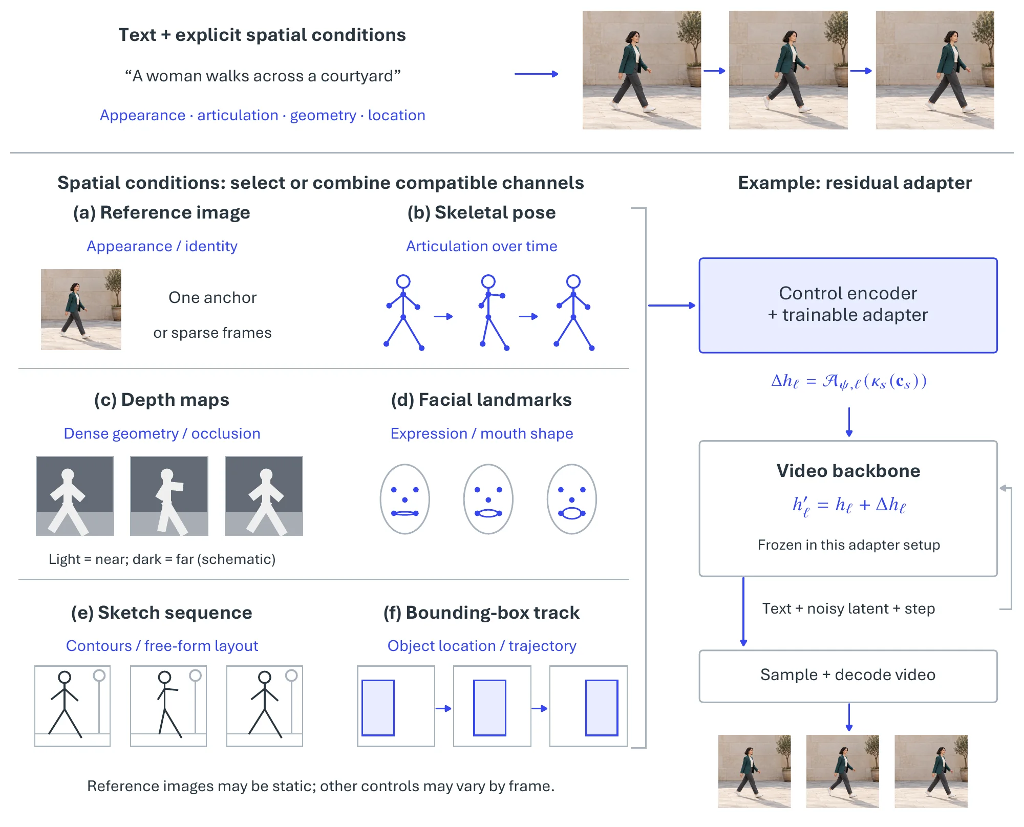
Image Control. A reference image (Figure 8.14a) specifies the style, content, or initial state of a video, which is the basis of animating a still and of keeping a subject’s appearance consistent. I2VGen-XL [2029], Stable Video Diffusion (SVD) [1873], VideoCrafter1 [2011], and Lumiere [2030] use the reference image as an initial condition, often by concatenating its latent with the initial noise, and ConsistI2V [2031] refines this for consistency. The model then generates a plausible motion sequence that evolves from the image, typically under a text prompt, as in DynamiCrafter [2032].
Pose Control. Pose-guided generation (Figure 8.14b) animates articulated subjects, predominantly humans, along a predefined sequence of skeletal poses, the video counterpart of pose-guided image generation [2033, 1693, 2034] and the core of avatar animation and character generation. The pose keypoints (e.g., , from MMPose [2035]) are encoded and injected at each denoising step, frequently through a ControlNet-style adapter [1693]. MagicAnimate [2036], Animate Anyone [2037], Follow-Your-Pose [2038], and DreamPose [2039] pair a reference image for appearance with a pose sequence for motion, DisPose [2040] disentangles the pose guidance, and Champ [2041] and MagicPose [2042] target high-fidelity motion, so that the output keeps the subject’s identity while following the target poses.
Depth Control. A sequence of depth maps (Figure 8.14c), estimated from an existing video or rendered from a 3D model, specifies dense 3D structure and so enforces consistent object layout and realistic occlusion. ControlVideo [2043], Make-Your-Video [2044], Control-A-Video [2045], and ControlNeXt [2046] adapt the ControlNet framework to video, processing each frame’s depth map with a trainable adapter that guides the denoiser; DreamDance [2047] and SparseCtrl [2048] also use depth for dynamic scene generation.
Landmark Control. Facial landmarks (Figure 8.14d) give fine-grained control over expression and are the standard interface for talking-head animation. EchoMimic [2049], HunyuanPortrait [2050], and LivePortrait [2051] animate a static portrait from landmarks, often themselves driven by audio, so that lip movements, blinks, and subtle expressions stay synchronized; TASTE-Rob [2052], Takin-ADA [2053], and Follow-Your-Emoji [2054] extend landmarks to more expressive control.
Sketch Control. Sketches (Figure 8.14e) let users define compositional layout and motion with simple line drawings, an intuitive interface for animation. ToonCrafter [2055], VidSketch [2056], AniDoc [2057], and SketchBetween [2058] take a sequence of sketches to guide interpolation or generation, encoding the line art and injecting it as a condition; LayerAnimate [2059] animates hand-drawn characters and scenes layer by layer, and MagicStick [2060] uses sketch-like structural cues for editing.
Bounding Box (BBox) Control. Bounding-box tracks (Figure 8.14f) specify where objects are and how they move over time, and dominate autonomous-driving simulation: MagicDrive [2061], DriveDreamer [2062], DriveScape [2063], and DreamForge [2064] use 3D boxes to control the position and motion of vehicles and pedestrians. The box information enters either through cross-attention, as in DiVE [2065], or as a spatial feature map, and Boximator [2066] and Ctrl-V [2067] generate and control object motion from box sequences.
Nearly every structural channel (pose, depth, sketch, box) is paired with an appearance reference image, since structure alone cannot fix identity or texture, and the channels cluster by application: image and landmark control in portrait and talking-head synthesis, pose and sketch control in character animation, depth and box control in geometry-faithful and driving-simulation settings.
8.3.2.3Benchmarks#
Unlike the text-to-video base case of §8.3.1, spatial control has no single canonical corpus or suite: each channel is trained and evaluated on data specialized to its application. Models are typically built on the general web-scale corpora of §8.3.1 (WebVid-10M [2024] and successors) for appearance priors, then specialized on task data: human-animation channels on dance- and fashion-video collections paired with extracted pose keypoints (e.g., , via OpenPose [526] or MMPose [2035]), talking-head landmark control on portrait-video sets, and bounding-box driving simulation on annotated driving datasets such as nuScenes [445], whose 3D box and trajectory labels supply the control signal directly.
Control-fidelity Metrics. Spatial control is judged on two axes simultaneously: the generic video-quality metrics of §8.3.1 (FVD [1950], CLIPSIM, and VBench [1951] dimensions) and channel-specific adherence metrics that measure how faithfully the output respects . The latter are necessarily per-channel: pose and landmark control report keypoint accuracy (re-detected-keypoint distance to the target skeleton or face mesh); depth control reports depth consistency between the re-estimated and the conditioning maps; image control reports identity and appearance preservation (face-/subject-similarity to the reference); and bounding-box control reports detection mAP and trajectory IoU of the generated objects against the conditioning boxes. Neither axis suffices alone, so methods report a quality-plus-adherence tuple: a model can maximize adherence by ignoring the prompt (rigid, texture-collapsed output) or maximize quality by ignoring the control. The same holds for every controlled axis that follows.
8.3.2.4Challenges and Trends#
Single-channel spatial control has three problems of its own; those that arise once several conditions are fused are discussed in §8.3.6. Because the structural scaffold and the appearance reference pass through the same denoiser, strong control leaks structure into texture: pose and depth conditioning induce identity drift or bake the scaffold’s silhouette into the surface, and disentangling what moves from what it looks like (as DisPose [2040] attempts for pose) remains open. Dense scaffolds (image, depth) over-constrain and suppress plausible motion, whereas sparse ones (boxes, coarse sketches) leave appearance and fine geometry ambiguous, so no channel is uniformly preferable and the right granularity depends on the task. And adapters trained on, say, frontal human dance transfer poorly to unusual viewpoints or non-human subjects, which is the data cost of per-channel specialization and one motivation for the multi-condition frameworks of §8.3.4.
8.3.3Temporal Controlled Video Generation#
Temporal control regulates how motion and timing evolve across frames, the lever behind cinematic camera work, narrative pacing, and believable physical interaction. It is the complement of the spatial scaffold of §8.3.2: where spatial control fixes where things are in each frame, temporal control fixes how they move between frames, externalizing the dynamics (object motion, camera path, timing) that the text-to-video base case of §8.3.1 otherwise had to sample blindly from a highly multi-modal motion posterior.
8.3.3.1Task Definition#
Temporal control instantiates Eq. (8.41) with an encoder of a motion or timing signal (an optical-flow field, an object trajectory, a camera-pose path, or a learned motion embedding),
| (8.48) |
The contrast with spatial control (Eq. (8.46)) is that constrains the inter-frame dynamics (how content moves between frames) rather than the per-frame appearance, so typically steers the temporal-attention or latent-warping pathway of the denoiser. The channels below differ in how the motion is specified: densely (optical flow), as object paths (trajectory), as virtual-camera parameters (camera), or as a transferable behavioral style (motion).
8.3.3.2Methodology#
The four channels specify inter-frame dynamics through different signals, and no single injection architecture serves them all. One implementation uses a trainable temporal-control branch to modulate features of a pretrained video backbone,
| (8.49) |
with dependence on noisy latents, diffusion step, and text omitted. More broadly, two routes recur: explicit transformations that use the motion to warp noise, latents, or attention features, and encoded conditioning that steers generation through adapters, attention, or learned motion features. They are not tied to particular channels (flow and trajectories can drive learned conditioning, and camera control can use geometry-aware warping), and Figure 8.15 keeps the four input channels separate from the two routes.
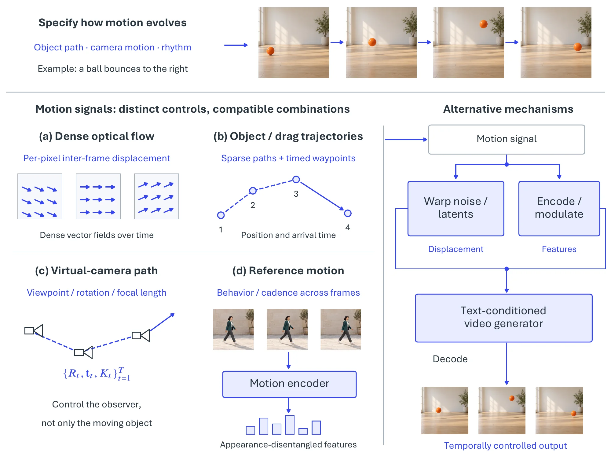
Flow Control. The most explicit motion signal (Figure 8.15a) is an optical-flow field, which records the per-pixel displacement between consecutive frames and so specifies dynamics at the finest granularity; conditioning on a sequence of such fields yields specific, coherent motion at the cost of authoring or estimating a dense signal. Motion-I2V [2068] integrates a motion-field predictor into its diffusion framework so that generation follows the supplied flow, I2VControl [2069] disentangles flow for unified control, and MOFA-Video [2070] animates a still image from user-painted motion fields. Go-with-the-Flow [2071] dispenses with the adapter altogether, warping the diffusion noise prior along the target flow so that the motion constraint lives in the sampling process rather than in an added branch.
Trajectory Control. Sparsifying the dense field into a few object paths (Figure 8.15b) trades pixel-level precision for an interface a user can actually author: a sequence of 2D or 3D coordinates, or a path drawn interactively, directs character movement or object kinematics, entering the denoiser either by modifying the latents or by steering cross-attention maps. MotionCanvas [2072], MagicMotion [2073], and Tora [2074] consume a predefined curve, FreeTraj [2075] relaxes this to free-form trajectories, Peekaboo [2076] also schedules when objects appear and disappear along the path, and DragNUWA [2077] and DragAnything [2078] let the user drag regions through the frame interactively. MotionCtrl [1811] handles object trajectory and camera motion in one controller, treating an object path and a camera path as two facets of the same inter-frame displacement.
Camera Control. Moving that displacement from objects to the observer (Figure 8.15c), camera-guided generation manipulates the virtual camera’s extrinsics (translation, rotation) and intrinsics (e.g., , focal length) to produce pans, tilts, zooms, and dolly moves. CameraCtrl [1810] and CameraCtrl II [2079] encode the camera trajectory as a conditioning feature; Direct-a-Video [2080], ViewCrafter [1812], and Cavia [2081] couple it with novel-view synthesis; and 3DTrajMaster [2082], MotionFlow [2083], and CineMaster [2084] control camera and objects jointly in 3D. Two directions now lead. ReCamMaster [2085] and TrajectoryCrafter [2086] re-render an existing monocular clip under a new camera path rather than generating from scratch, and Diffusion-as-Shader [2087] and GS-DiT [189] route the camera signal through a 3D proxy (a rendered shader pass or a pseudo-4D Gaussian field), which sharpens control by making it geometry-aware.
Motion Control. At the abstract end (Figure 8.15d), the signal is no longer a geometric displacement but a behavioral concept (walking, dancing, jumping) transferred from a reference video as a pose sequence or a learned motion embedding. Unlike the pose control of §8.3.2, it captures the dynamic style and cadence of a behavior rather than a frame-exact skeleton, so the central technical problem is disentanglement: extracting the motion while discarding the reference’s appearance. MotionDirector [2088], MotionClone [2089], and VMC [2090] learn this motion–appearance separation; Motion Prompting [2091], MotionAgent [2092], and MotionMatcher [2093] refine its granularity through trajectory- or feature-level motion descriptors; and DreamMotion [2094] and Customize-A-Video [2095] apply a reference clip’s dynamics to a new subject or scene fixed by the text prompt.
The channels trade precision against ease of specification: dense flow gives pixel-accurate control but is laborious to author, a motion embedding is effortless to supply but steers the result only loosely, and the most usable systems therefore pair an abstract signal (a drawn path, a reference clip) with a learned predictor that densifies it into the flow- or latent-level displacement the backbone actually consumes.
8.3.3.3Benchmarks#
As with spatial control (§8.3.2), temporal control has no single canonical suite: each channel is evaluated against data specialized to its signal. Models build on the general corpora of §8.3.1 for appearance and motion priors, then evaluate on task-specific resources: camera control on the posed-video collection RealEstate10K [734], whose per-frame camera poses supply both the conditioning signal and the evaluation ground truth, increasingly supplemented by the larger and more scene-diverse DL3DV-10K [735] to test generalization beyond real-estate walkthroughs; flow control against the MPI-Sintel optical-flow benchmark [956] or flow re-estimated from generated clips with RAFT [255]; and motion- and trajectory-control quality through the motion-smoothness and dynamic-degree dimensions of VBench [1951].
Control-fidelity Metrics. Alongside the generic video-quality metrics of §8.3.1, each channel measures adherence by re-extracting the control signal from the generated clip and comparing it with the conditioning input; the estimator and the error differ per channel.
Flow adherence. The optical flow of the generated clip is re-estimated with RAFT [255] and compared to the conditioning flow by the end-point error (EPE), the per-pixel displacement difference averaged over pixels and frames. A complementary flow-warping error warps each generated frame onto the next with the target flow and reports the photometric residual, which tests whether the rendered motion realizes the commanded displacement rather than merely correlating with it.
Trajectory adherence. The controlled object is re-localized in the output with a dense point tracker such as CoTracker [2096] or a detector, and its tracked center is compared to the target path by the mean distance, normalized by frame size and averaged over time and instances; this is the object motion-control error reported by Tora [2074] and DragNUWA [2077], and it penalizes both spatial deviation and mistimed arrival.
Camera adherence. The camera trajectory of the generated clip is recovered by structure-from-motion (COLMAP [115]) and aligned to the target up to a similarity transform, since pose is recoverable only up to scale. Following CameraCtrl [1810], a rotation error (the geodesic angle between estimated and target rotations, summed over frames) and a translation error (the distance between scale-normalized camera centers) are reported; failure to reconstruct a stable trajectory at all is itself diagnostic of an incoherent output.
Motion-transfer fidelity. With no ground-truth video, fidelity is measured from two sides: a motion-similarity term compares the dynamics of output and reference (the correlation of tracked point trajectories or temporal feature statistics), and an appearance-divergence term (CLIP similarity to the new prompt together with low feature similarity to the reference’s appearance) confirms that the subject was re-synthesized rather than copied.
As for spatial control, these adherence errors are reported together with generic quality, since a near-static clip trivially minimizes EPE and pose error while ignoring the prompt.
8.3.3.4Challenges and Trends#
Three problems are specific to temporal control; fusing it with other conditions is discussed in §8.3.6. Because the motion signal passes through the same backbone that renders appearance, a transferred motion often drags the source clip’s identity or texture with it, the leakage that MotionDirector [2088] and VMC [2090] try to disentangle and that remains unsolved for large appearance gaps between reference and target. Dense flow over-constrains and suppresses generative freedom, whereas a single trajectory or a short reference clip under-specifies the global dynamics, which is why methods increasingly interpose a learned predictor that densifies an abstract signal into a flow- or latent-level field. And a commanded camera path or object trajectory can demand views or dynamics inconsistent with the scene geometry, producing parallax errors and object distortion; 3D-aware camera control (ViewCrafter [1812], CineMaster [2084]) routes the control through an explicit geometric proxy for exactly this reason, which links temporal control back to the volumetric representations of §8.2.
8.3.4Other Controlled Video Generation#
Beyond the spatial scaffolds of §8.3.2 and the motion signals of §8.3.3, a video can be steered by further, application-specific conditions: an artistic style reference, a handful of draggable points, a bird’s-eye-view road layout, a target text string to render, or a synchronizing audio track. Each externalizes an attribute that text specifies only loosely, extending controllable generation to creative, interactive, and domain-specific settings; together they raise the question the single-axis interfaces leave open, how to honor several conditions at once, which the universal frameworks at the end of this subsection try to answer.
8.3.4.1Task Definition#
Taken one at a time, each “other” modality instantiates the generic conditional sampler of Eq. (8.41) with an encoder of a heterogeneous control signal (a style reference, a set of draggable points, a BEV layout, a target text string, or an audio track). The distinctive task of this subsection, however, is to honor several such conditions simultaneously: universal and multi-task frameworks fuse encoded signals into a single sequence,
| (8.50) |
so that the encoded conditions are processed jointly rather than one axis at a time, with recovering the single-modality case and for all recovering the text-to-video base case of §8.3.1.
8.3.4.2Methodology#
The methods fall into single-modality channels (style, points, BEV, text rendering, audio) and multi-task frameworks that combine compatible conditions. Writing , the common interface is
| (8.51) |
where is a model-specific conditioning interface that may act at several layers rather than produce one fixed-size embedding. Three implementations are representative and can be combined: summed adapter residuals , concatenation of the encoded channels with the model input or features, and unified attention over condition tokens. Figure 8.16 shows the five input modalities and these three fusion designs; denotes one selected modality and a supported combination.
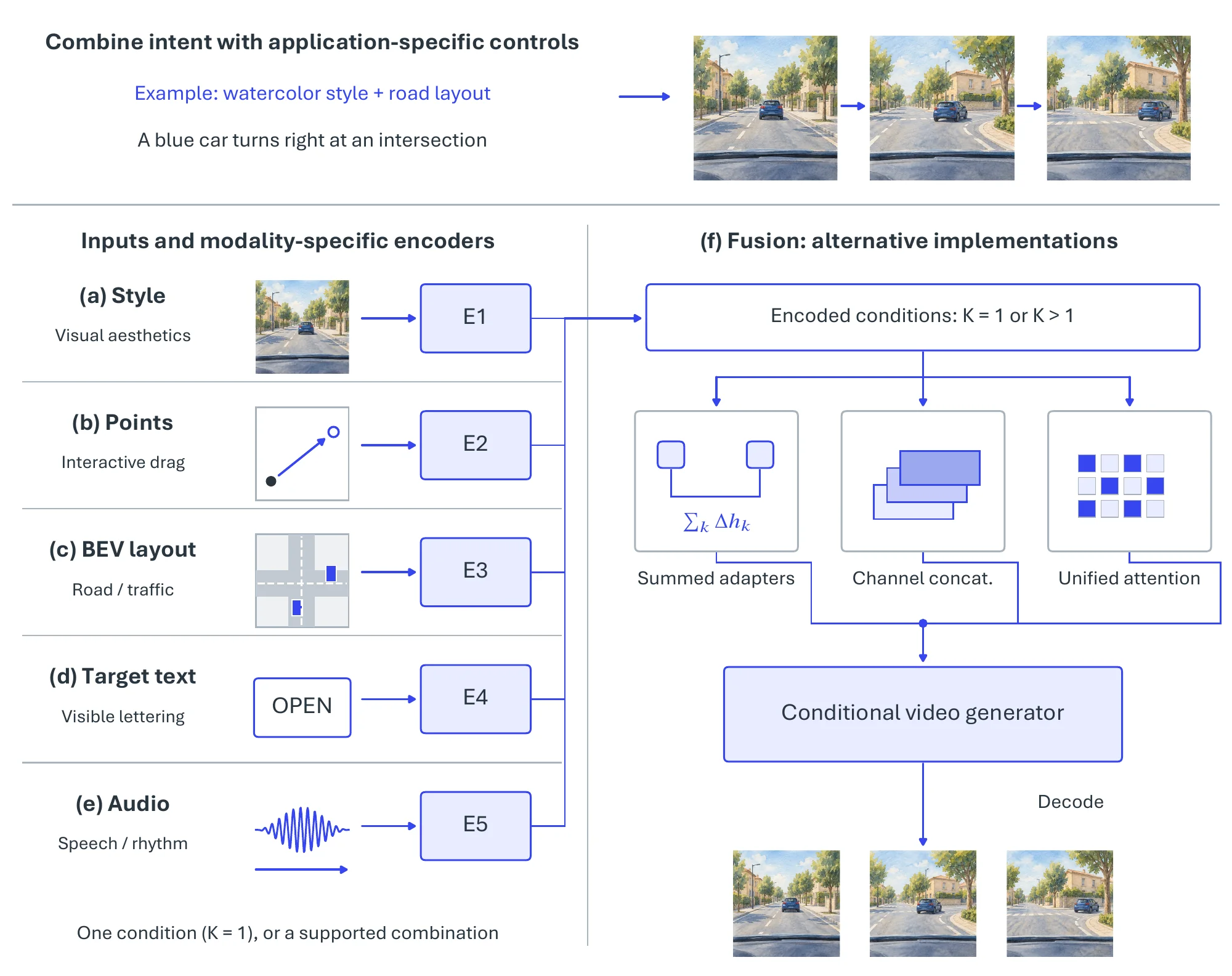
Style Control. Style-guided generation transfers the artistic style of a reference image or video to a target video. Per-frame style transfer flickers; diffusion-based approaches such as Rerender A Video [2097], StyleCrafter [2098], FRESCO [2099], and StyleMaster [2100] instead integrate the style into generation, often by guiding it with the CLIP embedding of the style reference so that the style holds across frames, and UniVST [2101] generalizes this into a universal framework. FrameGuidance [2102] and OmniVDiff [2103] add training-free frame-level guidance and omni-controllable diffusion, respectively.
Point Control. Point control fixes motion through a sparse, interactive interface: the user drags a few points on an object from an initial frame to a new position in a later frame, and the model infers a plausible motion for the whole object. Drag-A-Video [2104] introduced the approach by optimizing latent codes to satisfy the point constraints, Track4Gen [2105] focuses on tracking the user-specified points robustly, and the 3D-aware camera controllers of §8.3.3 [2087, 189] also accept sparse point input for non-rigid manipulation.
Bird’s-Eye View (BEV) Control. BEV-guided generation serves autonomous-driving simulation: a sequence of top-down semantic maps dictates the road layout, the positions of other vehicles, and the movements of pedestrians. DriveDreamer-2 [2106], MagicDrive-V2 [2107], DiVE [2065], DreamForge [2064], and Panacea [2108] take these maps as input and generate first-person driving video consistent with the specified layout and dynamics.
Text Rendering. Many generators cannot render coherent, legible text inside a scene, so a dedicated channel treats the target string itself as the control signal. Text-Animator [2109] adds text-embedding injection and refinement modules that improve the structure and temporal stability of rendered text, and Wan [1990] reports being the first video foundation model able to render legible Chinese and English text.
Audio Control. Audio-controlled generation synthesizes video synchronized with an input audio signal, in two sub-domains. Voice-guided generation produces talking heads: EMO [2110], VASA-1 [2111], DreamTalk [2112], and AniPortrait [2113] take a reference image and a speech clip, extract audio features with a pretrained encoder, and drive facial motion with accurate lip-sync and expression; Say Anything [2114], MuseTalk [2115], and CAFE-TALK [2116] focus on high-fidelity lip synchronization, and V-Express [2117] and MegActor [2118] balance audio against other control signals. Sound-guided generation follows more general audio such as music or ambient sound, using its rhythm, pitch, and emotional tone to drive visual elements, motion, and scene transitions: TA2V [2119], MotionCraft [2120], AV-Link [2121], and ASVA [2122] generate music visualizations or scenes that follow the energy and structure of a track, and MagicInfinite [2123] and Sound2Sight [2124] explore more open-ended audio-driven generation.
Universal and Multi-Task Control. The single-modality channels each add one encoder; universal frameworks realize the fusion of Eq. (8.50) in a single model, along two lines. Autoregressive models built on multimodal large language models generate video from discrete visual tokens, as in VideoPoet [2125] and Emu3 [2003]. Diffusion models are being adapted to many conditions at once: VideoComposer [2126] integrates depth, pose, motion, and other conditions by channel concatenation, OmniHuman [2127] generates human video under multiple controls by mixing cross-attention and concatenation, and FullDiT [2128] processes all conditions with unified attention, the third realization of .
8.3.4.3Benchmarks#
Being heterogeneous, the “other” modalities share no single suite: each is evaluated against data and metrics specialized to its signal, with the general corpora of §8.3.1 supplying the appearance and motion priors. BEV control is evaluated on driving collections such as nuScenes [445], whose paired BEV layouts and front-camera footage furnish both the conditioning signal and the ground truth. Voice-guided talking-head generation is evaluated on portrait-video collections (HDTF [2129] and VFHQ [2130] are standard) and sound-guided generation on audio–video corpora with aligned music or ambient tracks. Style and point control, having no canonical benchmark, are assessed on the general corpora plus qualitative and user studies.
Control-fidelity Metrics. Beyond the generic video-quality metrics of §8.3.1 (FVD [1950], CLIPSIM, and VBench [1951] dimensions), each modality adds an adherence metric tailored to its signal, reported together with generic quality as in §8.3.2. Style adherence combines a CLIP style-similarity to the reference with a temporal-consistency term that penalizes flicker. Point adherence re-localizes the dragged keypoints in the output and reports their deviation from the target path, as in the trajectory metric of §8.3.3. BEV adherence renders or detects objects in the generated clip and reports detection-mAP and layout-IoU against the input map. Text adherence runs OCR on the rendered frames and reports recognition accuracy and legibility. Audio adherence measures lip-sync quality with SyncNet-style confidence and landmark error for voice, and audio–visual synchrony for sound.
8.3.4.4Challenges and Trends#
The central difficulty here, fusing conditions of incommensurate dimensionality and strength without one washing out or dominating the others, is shared with the spatial and temporal axes and discussed in §8.3.6. Two problems are specific to these modalities. Text rendering must keep glyphs legible and stable at once, and per-frame legibility and temporal coherence pull against each other as the camera or the text moves. BEV control covers a narrow domain: models trained on a handful of driving datasets inherit their sensor rigs, cities, and traffic statistics, and generalize poorly beyond them.
8.3.5Video Editing#
Video editing takes an existing clip and modifies it under user instruction, rather than generating one from scratch (§8.3.1) or steering that generation with controls (§8.3.2–§8.3.4). It is the temporal lift of the image editing of §8.1.3, and its defining demand is selective preservation: the operator must change only the targeted content while holding the source’s geometry, layout, and motion fixed across every frame, so the central technical problem is to balance editability against spatio-temporal consistency without artifacts or unintended drift.
8.3.5.1Task Definition#
Given a source clip encoded as and an edit instruction , an editing operator
| (8.52) |
returns an edited clip that applies the requested change while preserving unedited content and the source motion, recovering the image editing operator of Eq. (8.8) exactly at . Eq. (8.52) encodes two competing objectives: editability (the output must realize the instruction ) and preservation (the unedited regions and the source dynamics must survive untouched).
8.3.5.2Methodology#
The five paradigms are overlapping choices of training strategy and preservation mechanism: training-free editing keeps the weights fixed, one-shot tuning updates selected parameters on the source clip, trained instruction editors learn across editing data, attention-based editing reuses or modifies source attention, and structural guidance conditions the edit on source-derived depth, edges, or poses. Many of them share a diffusion recipe that inverts the source clip and re-denoises it under the instruction; writing for DDIM inversion of the pretrained or adapted backbone of §8.3.1,
| (8.53) |
where denotes the terminal diffusion step, distinct from the clip length . Inversion supplies a source-correlated initialization; how much of the source survives then depends on the sampling, feature reuse, and guidance applied during re-denoising. Figure 8.17 schematizes the five paradigms, with panels (a)–(e) keyed to the paragraphs below.
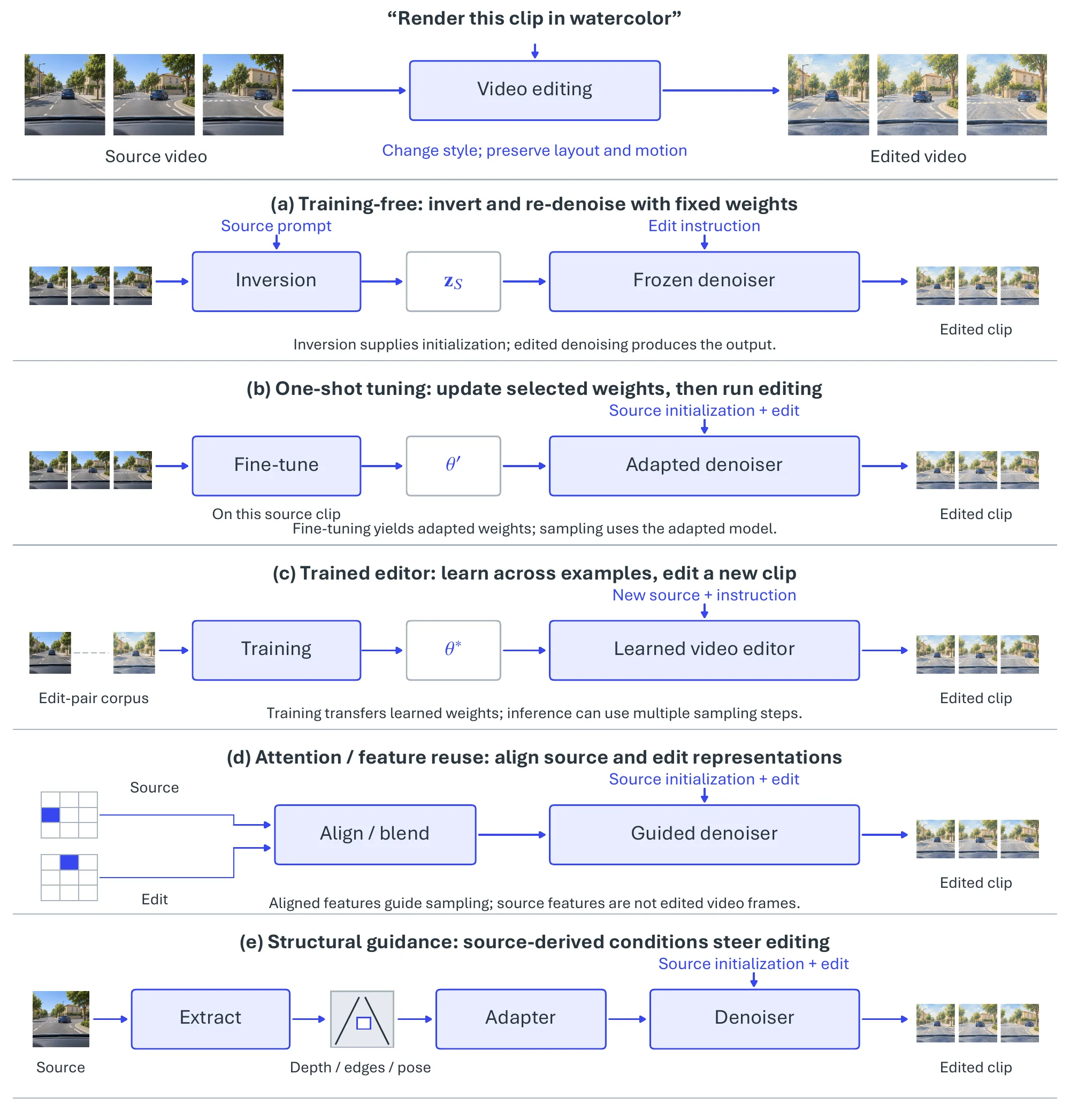
Training-Free (Zero-Shot) Methods. The lightest realization of Eq. (8.53) (Figure 8.17a) edits a video without any fine-tuning, analogous to zero-shot image editing [2131]: DDIM inversion encodes the source into latent codes and noise maps, and the denoising process is rerun on them under the edited prompt. Text2Video-Zero [2132] and Pix2Video [2133] established the category, and vid2vid-zero [2134], I2VEdit [2135], RAVE [2136], and FastVideoEdit [2137] add latent-code warping and feature injection to improve temporal consistency without fine-tuning.
One-Shot Tuning Methods. Trading a little training for sharper fidelity (Figure 8.17b), Tune-A-Video [2014] fine-tunes a limited subset of a pretrained text-to-image diffusion model’s parameters on the frames of a single source video, so that the model learns its content and motion and can regenerate it under a new prompt. Dreamix [2138] builds on one-shot fine-tuning to improve both editability and fidelity to the original motion.
Training-Based Methods. The limited control and quality of inference-time editing have motivated editors that learn a reusable operator from editing data (Figure 8.17c), particularly for instruction-based editing. InsV2V [2139] extends the InstructPix2Pix [1711] framework directly to video; GenProp [2140] propagates an edit from a user-modified first frame to the rest of the sequence; and VideoPainter [2141] uses a video inpainting model as an intermediary. UNIC [2142] handles many editing tasks in one model by concatenating the conditions into a sequence with task-aware positional embeddings, and EditVerse [2143] unifies video generation and editing by representing text, image, and video as one token sequence processed with self-attention, which permits in-context learning and flexible inputs.
Attention-Based Editing. To protect preservation within the inference-time recipe (Figure 8.17d), many techniques manipulate the cross-attention maps directly: following Prompt-to-Prompt in images, they blend the attention maps of the original and edited prompts so that the inverted source structure of Eq. (8.53) survives the re-denoising. FateZero [2144] and Video-P2P [2145] were early examples, and Edit-A-Video [2146], TokenFlow [2147], UniEdit [2148], and AnyV2V [2149] improve temporal consistency at the token or feature level, enabling localized edits such as changing an object’s material or color while the scene structure is kept.
Editing with Structural Guidance. At the explicitly guided end (Figure 8.17e), editing is conditioned on spatial signals extracted from the source video, the conditioning machinery of §8.3.2 repurposed for preservation rather than generation. Rerender A Video [2097] feeds the source’s depth or edge maps to a ControlNet-like module during editing so that geometry and layout stay intact, and MagicEdit [2150] accepts a variety of spatial inputs (e.g., , pose, sketches, segmentation maps) for high structural fidelity, which suits style transfer and object replacement, where preserving structure is what prevents distortion and keeps motion coherent.
The paradigms trade cost against control: training-free editing avoids per-clip weight updates but may still need iterative inference, whereas a trained instruction editor is expensive to build but generalizes across edits.
8.3.5.3Benchmarks#
Video editing has no single canonical suite, and evaluation has moved from shared source-video collections toward purpose-built, fine-grained editing benchmarks. Early evaluations report on DAVIS [987], the de facto source set for object-centric edits, and on the LOVEU text-guided video-editing (TGVE) benchmark [2151], which supplies prompt–clip pairs with human ratings; VPBench, released with VideoPainter [2141], adds masked clips with dense captions for inpainting-style edits. The most recent suites target instruction-guided editing and pair richer data with model-based scoring. FiVE [2152] contributes real clips (drawn from DAVIS) and generated clips across six fine-grained editing types, with object-level prompt pairs and masks, evaluated under a -metric protocol spanning background preservation, text–video similarity, temporal consistency, video quality, and runtime. IVEBench [2153] scales this to source videos spanning seven semantic dimensions and clip lengths from to frames, across eight task categories ( subcategories) whose prompts are generated by LLMs and refined by experts, and adopts a three-dimensional protocol (video quality, instruction compliance, and video fidelity) that fuses traditional metrics with multimodal-LLM-based assessment.
Editing-fidelity Metrics. Editing is judged on three axes that mirror the editability–preservation tension of Eq. (8.52). The classic metrics are, for edit adherence, the CLIP similarity between each edited frame and the target prompt; for temporal consistency, frame-to-frame CLIP similarity together with a warping error that flow-aligns adjacent frames and reports the photometric residual; and for structure and background preservation, PSNR / SSIM / LPIPS on the unedited regions against the source, atop the generic FVD [1950] quality score. These scalars correlate only loosely with human judgment on fine-grained edits (an object recolored but mislocalized can still score well), so the latest benchmarks add vision-language judges: FiVE-Acc [2152] uses a VLM to test whether the intended fine-grained edit succeeded, and IVEBench [2153] scores instruction compliance and fidelity with multimodal LLMs alongside the traditional metrics. Results are reported as an edit-versus-preservation pair, since ignoring the instruction trivially maximizes preservation.
8.3.5.4Challenges and Trends#
Three problems are specific to editing. Pushing the edit harder erodes the unedited regions and the source motion, while protecting them too strongly suppresses the requested change; this editability–preservation trade-off of Eq. (8.52) is what every paradigm above negotiates differently. The invert-and-re-denoise recipe of Eq. (8.53) is imperfect, and its reconstruction error compounds over long clips, so edits that are clean over a few seconds degrade over minute-scale video. And training-based editors follow only the edit types seen in their training pairs, so a flexible instruction editor that handles arbitrary edits remains open; the unified generate-and-edit models UNIC [2142] and EditVerse [2143], which treat the source clip as one stream among many in shared attention, are the current attempt.
8.3.6Summary and Critical Challenges and Future Directions#
Table 8.9 places the five control axes side by side: the control signal each introduces, the operator it instantiates over the shared sampler of Eq. (8.41), the paradigms it surveys, the methods anchoring each, and the benchmarks on which it reports.
| Control axis | Control signal / operator | Dominant paradigms | Canonical methods | Benchmarks / metrics |
| §8.3.1 Text-to-video | Text only, ; (Eq. (8.42)) | GAN; autoregressive token; diffusion / diffusion transformer | CogVideo, Sora, Wan, HunyuanVideo, Cosmos | UCF-101, MSR-VTT, VBench, EvalCrafter; FVD, CLIPSIM |
| §8.3.2 Spatial control | Per-frame scaffold (Eq. (8.46)); residual injection (Eq. (8.47)) | Image, pose, depth, landmark, sketch, bounding box | Animate Anyone, MagicAnimate, ControlVideo, EchoMimic, MagicDrive | nuScenes, pose-annotated video; keypoint / depth / identity / detection adherence |
| §8.3.3 Temporal control | Motion signal (Eq. (8.48)); temporal-branch injection (Eq. (8.49)) | Flow, trajectory, camera, motion; latent warping or encoded conditioning | Motion-I2V, Tora, DragNUWA, CameraCtrl, MotionDirector | RealEstate10K, DL3DV-10K, MPI-Sintel; EPE, path / pose error, transfer fidelity |
| §8.3.4 Other control | Heterogeneous fused by (Eqs. (8.50), (8.51)) | Style, point, BEV, text, audio; summed adapters, concatenation, unified attention | StyleCrafter, DriveDreamer-2, EMO, VideoComposer, FullDiT | nuScenes, HDTF, VFHQ; style / point / BEV / OCR / lip-sync adherence |
| §8.3.5 Video editing | Existing clip edit intent edited clip; (Eq. (8.52)) | Training-free, one-shot tuning, trained instruction editors, attention reuse, structural guidance | Tune-A-Video, TokenFlow, InsV2V, UNIC, EditVerse | DAVIS, LOVEU-TGVE, FiVE, IVEBench; edit-vs-preservation tuple, VLM / MLLM judges |
The axes partition not by output domain, since all five decode a clip from the same , but by the control fed to one shared sampler: text-to-video is the limit, spatial, temporal, and other control progressively enrich , and editing alone reverses the direction of the map, taking an existing clip in place of pure noise. The injection mechanism converges across axes: the spatial residual branch (Eq. (8.47)), the temporal branch (Eq. (8.49)), and the multi-condition interface (Eq. (8.51)) are one idea, a trainable control pathway added to a pretrained backbone, generalized from one condition to many, and the most recent systems (VideoComposer, FullDiT, UNIC, EditVerse) go further by folding every axis, editing included, into a single token sequence processed by shared attention. Evaluation has not converged: no suite spans the five axes, each reports generic quality together with a channel-specific adherence score, and the newest editing benchmarks (FiVE, IVEBench) add vision-language and multimodal-LLM judges to improve human alignment.
Video generation inherits every difficulty of the 2D and 3D priors of §8.1 and §8.2 and adds the time axis, which turns several already-hard problems into open ones; the four below cut across all five axes.
Temporal coherence and long-horizon drift. The defining difficulty of video over image generation is keeping content stable across frames. The signature artifact is flicker, the high-frequency appearance instability between adjacent frames that plagues per-frame and early GAN-based methods (§8.3.1); over longer spans it gives way to identity drift, the gradual mutation of a subject’s appearance, color, or fine texture across a clip; and in autoregressive roll-outs to error accumulation, the compounding of small per-step mistakes that caps usable clip length. Latent video autoencoders with temporal compression [1873, 2007] and dedicated spatio-temporal attention suppress flicker, while autoregressive–diffusion hybrids such as CausVid [2004] and MAGI-1 [2005] combine sequential consistency with diffusion fidelity to push toward minute-scale generation; coherence over arbitrarily long horizons remains unsolved and is the binding constraint on the world-model applications that motivate the section.
Controllability versus fidelity under multi-condition fusion. As §8.3.2–§8.3.4 stack heterogeneous conditions (spatial scaffolds, camera paths, audio, style) onto Eq. (8.41), the conditions begin to conflict. Over-strong conditioning yields rigidity and texture collapse; weak conditioning ignores the control; and naive fusion produces control-signal dilution (summed adapters wash one another out), condition leakage across frames, and collapse to the dominant condition when one modality (e.g., , audio in talking-head generation) overwhelms the rest. Compositional and universal frameworks (VideoComposer [2126], OmniHuman [2127], and the unified-attention design of FullDiT [2128]) replace per-axis injection with joint token fusion and task-aware positional embeddings, but a principled account of how to weight and arbitrate competing conditions is still missing.
Physical and 3D plausibility. Even a temporally coherent, well-controlled clip may depict an impossible world, which is the bridge back to §8.2. Generated motion frequently violates object permanence (objects teleport, morph, or vanish), contact and rigid-body dynamics (rigid objects warp non-rigidly; feet slide; occlusions resolve implausibly), and multi-view consistency under camera motion, where the same scene is rendered inconsistently from successive viewpoints. Systems presented as steps toward “world simulators”, Sora [1991] among them, still exhibit these failures on closer inspection. Camera-control methods [1810, 1812] and explicitly 3D-aware video diffusion (Diffusion-as-Shader [2087] and GS-DiT [189]) narrow the gap by conditioning generation on geometry, which suggests that the more promising route to physical plausibility runs through the volumetric representations of §8.2 rather than through scale alone.
Compute, latency, and evaluation. Underlying all three is cost: a spatio-temporal latent is an order of magnitude larger than an image latent, so long, high-resolution clips strain memory and make iterative sampling slow, which in turn limits the context length available for coherence and the conditioning budget available for control. Consistency distillation and few-step samplers, together with sparse and causal attention, are the active responses. Evaluation compounds the problem: distributional scores such as FVD and per-frame FID are blind to temporal and control adherence, and automatic metrics correlate weakly with human judgment, so reported progress is hard to compare across methods; benchmarks and human-aligned protocols that jointly score fidelity, temporal coherence, and per-axis control adherence are a central near-term need.
Coherence and physical plausibility both demand longer temporal context, which inflates compute, and every added condition enlarges the evaluation surface, so progress on any one of the four is bounded by the others. Together they mark the last step of the progression traced across §8, from the static 2D prior of §8.1 through the static volumetric prior of §8.2 to dynamic, navigable models that consume spatial structure over time.