The 4D representations extend the 3D representations of Section 4.2 into the temporal dimension, modeling not only the geometry and appearance of a scene at a single instant but also how both evolve over time. They are the substrate for tasks that involve dynamic content (moving objects, deformable bodies, fluid simulation, novel-view synthesis of casually captured videos), where a sequence of independent 3D reconstructions would either fail to maintain temporal coherence or be prohibitively expensive to recompute frame by frame.
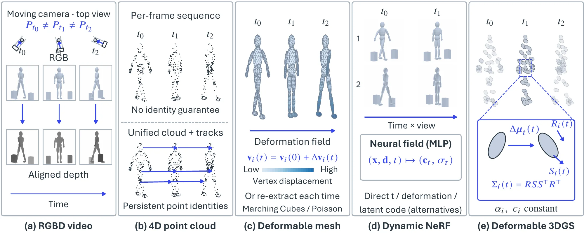
We organize this section around five 4D representations (Figure 4.4), each obtained by adding time to one of the 3D representations of Section 4.2: RGBD video, point clouds, meshes, neural radiance fields, and deformable 3D Gaussian Splatting. The voxel and implicit-field families of Section 4.2 admit analogous time extensions but are less commonly used in the 4D literature, and we therefore omit them as standalone subsections here.
4.3.1RGBD Video#
RGBD videos , with and , are a straightforward extension of RGBD images (see Section 4.2.1) to the temporal domain. Equivalently, they can be stored as a 4D tensor , with the last channel holding depth. RGBD videos can be captured using depth sensors, such as Microsoft Kinect or Intel RealSense, which provide synchronized RGB and depth data. These videos are commonly used in applications such as motion capture, gesture recognition, and augmented reality. There are also many learning-based methods [293, 294, 295] that directly predict consistent RGBD videos from monocular video sequences . However, such a representation may struggle to handle complex dynamic scenes with significant occlusions or topology changes. If we want to further reconstruct a unified 4D scene in a canonical space, we may also need to provide or estimate camera poses for each frame, as well as point trajectories over time to establish temporal correspondences, e.g., via joint pose-trajectory optimization in recent video-based SfM systems [296].
4.3.2Point Cloud#
Point clouds are another popular representation for 3D scenes (see Section 4.2.3), and they can be extended to 4D by incorporating temporal information. A 4D point cloud can be represented as , where is the 3D position of point at time step , and is the corresponding color. To map an uncalibrated, continuous video sequence , to a 4D point cloud representation, it generally has two types of representations: (1) a sequence of point clouds in a fixed coordinate system, where each is an independent point cloud at time step ; (2) a unified point cloud , where is the total number of points across all time steps, and each point has a trajectory over time. The first representation is easier to obtain, as it can be directly derived from the depth maps estimated from each frame using monocular depth estimation methods [296]. However, it may suffer from temporal inconsistencies and a lack of point correspondences across frames. The second representation, in contrast, requires explicit temporal correspondences (either ground-truth tracks, optical-flow lifting [255], or jointly optimized point trajectories [296]), and is therefore harder to acquire, but it offers persistent point identities and consistent trajectories that are useful for downstream 4D reconstruction, motion analysis, and dynamic NeRF/3DGS initialization.
4.3.3Mesh#
We can extend the mesh representation (see Section 4.2.4) to 4D by representing a sequence of 3D meshes over time. A 4D mesh is a sequence with , where and are the vertices and faces of the mesh at time , respectively. To reconstruct a 4D mesh using deep learning, researchers typically sample a set of points on the mesh surface at the original time step , and then learn a deformation field to model the motion of these points over time [297]. Then, the deformed points at each time step can be used to reconstruct watertight manifold meshes using Marching Cubes [105] or Poisson Surface Reconstruction [298].
4.3.4NeRF#
As discussed in Section 4.2.6, NeRF [119] is a continuous, volume-based 3D representation that maps a 3D position and a 2D viewing direction to a color and a volume density via a learned function . This function is typically implemented using a neural network, which is trained on a set of input images and their corresponding camera poses. To extend NeRF to dynamic scenes, we can introduce a temporal dimension to the input of the function, resulting in a 4D representation . This allows the model to capture changes in the scene over time, enabling the rendering of novel views at different time steps. In practice, the temporal dimension can be represented in various ways. For example, it can be trained to directly take a continuous time variable as input, and output displacement to deform the 3D position at time step [187]. Alternatively, the deformation can be parameterized using a dense field [299], which models the rigid transformations (rotation and translation) of points in the scene over time. Other approaches [300] may also incorporate additional latent codes to represent different time steps, enabling the model to capture more complex temporal variations.
4.3.5Deformable 3D Gaussian Splatting#
Given a static scene representation , which contains 3D Gaussians [121] (see Section 4.2.7), where is the opacity, is the mean (3D position), is the covariance matrix, and is the color function that maps a viewing direction to an RGB color, we extend it to a deformable 3D Gaussian Splatting representation for dynamic scenes by letting both the mean and the covariance vary in time: [191]. The mean is parameterized by a deformation field, , where is the initial position at and is the time-dependent offset. The covariance is decomposed in the same way as in the static case, , with the rotation and scaling themselves outputs of the deformation field at time . The opacity and color function are typically kept constant over time. In practice, this means that the appearance of the scene does not change significantly over time, while the latest work [301] also explores time-varying colors and opacities. This representation allows for efficient rendering of dynamic scenes by accounting for the temporal changes in the positions and shapes of the 3D Gaussians.