Learning-based spatial reasoning refers to the class of methods that acquire and perform spatial reasoning from data, rather than from the hand-authored geometric, mechanical, or symbolic models surveyed in §7.1. The six subsections that follow are ordered by the locus of the structural prior: it begins inside the learned representation (latent feature interaction, explicit programs, hard-coded symmetries, optimization layers in the forward pass), moves to the agent’s action-conditioned behavior (reinforcement learning with spatial inductive biases), and ends with joint decision-making across coordinated agents.
7.2.1Implicit Neural Spatial Reasoning#
We define implicit neural spatial reasoning as the family of neural approaches in which spatial relations are encoded in learned feature representations, attention patterns, latent object interactions, or architectural inductive biases, rather than specified through hand-written rules, symbolic programs, or fully explicit relational graphs. Implicit does not mean that these models never use boxes, masks, object proposals, or task-level labels; it means that the reasoning procedure itself is never given as a symbolic program, so the model must learn spatial dependencies from end-to-end or weakly structured supervision. Several families below (latent scene graphs, capsule networks) expose partly inspectable structure, yet remain implicit in that their relational structure is learned or emergent rather than supervised. Figure 7.7 shows the representative tasks.
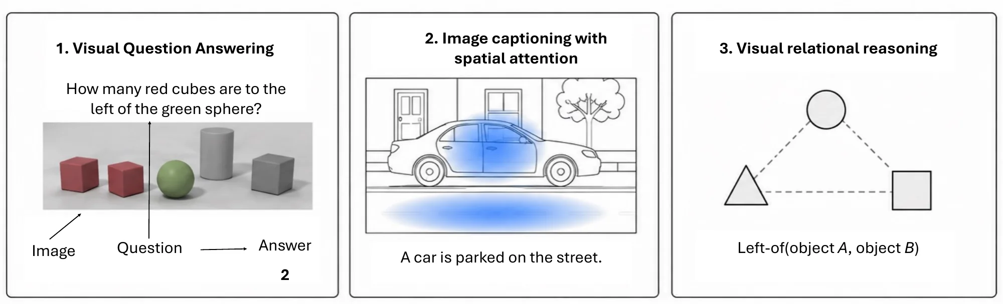
7.2.1.1Task Definition#
Given one or more images , optionally paired with a language query or task goal (and possibly boxes, masks, or proposals as features), an implicit reasoner computes a latent spatial representation and a task output,
| (7.18) |
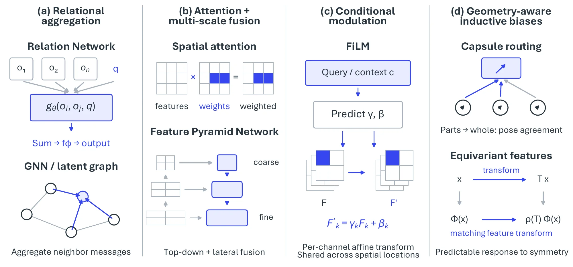
where encodes the relations relevant to the task and is an answer label, a caption, or a relation label. Supervision reaches the model only through ; the relational structure inside is never annotated, so it must emerge from end-to-end training. The methods below differ in the mechanism by which is formed (Figure 7.8).
7.2.1.2Methodology#
Relational Aggregation over Latent Objects. The most direct approach treats a set of feature vectors as latent “objects” and learns to aggregate their interactions. Relation Networks (RN) [1349] score every pair: given objects (e.g., , feature vectors from spatial regions of a CNN map) and an optional query ,
| (7.19) |
where produces a query-conditioned relation embedding for each pair and maps the sum to the task output. Considering all pairs forces the network to learn pairwise spatial and semantic relations, at cost in the number of objects. Graph neural networks and latent scene graphs generalize this from a complete graph to a learned, sparser topology, with proposals or feature regions as nodes and learned edges as spatial dependencies; iterative message passing for scene-graph generation [798] alternates between refining node features and updating relation embeddings, learning the topology end-to-end. Such models are the clearest semi-explicit case in this subsection: the graph is inspectable and often trained with relation annotations (e.g., , from Visual Genome), yet the intermediate relational representation is learned rather than specified by a program, and its quality is bounded by the upstream proposal stage.
Spatial Attention and Multi-Scale Feature Fusion. A second family controls where and how strongly the model attends across the spatial layout, and fuses evidence across scales, rather than scoring all pairs. CNN spatial attention weights locations in a feature grid, from the hard and soft attention of Xu et al. [1350] for captioning and grounded VQA [1351] to SCA-CNN’s joint spatial and channel attention [1352]; vision transformers make relating image parts intrinsic through self-attention over patches [142], with locality-aware variants (Swin [469], PVT [1353], Twins [1354]) trading global receptive field for cost; and Feature Pyramid Networks [597] add a top-down pathway so that a relation coupling a fine object with a coarse region (a car “on” a street) can be read from one map. These designs are representation backbones that preserve and aggregate spatial information for the reasoning built on top of them, not reasoning modules in themselves.
Conditional Feature Modulation. A third family conditions one representation on another rather than aggregating or attending. In FiLM (Feature-wise Linear Modulation) [1355], a conditioning vector (e.g., , an encoded query or global context) predicts affine parameters that are applied feature-wise to a target map, so the same backbone can be steered per task. For a query like “What is to the left of the green cube?”, a FiLM layer can learn to amplify features to the left of regions identified as the green cube, making reasoning adaptive and context-dependent.
Geometry-Aware Inductive Biases. A fourth family bakes geometric regularities into the architecture, trading data-driven flexibility for sample efficiency where the relevant geometry is known. Capsule Networks [1356] replace scalar activations with vector-valued capsules whose orientation encodes instantiation parameters (pose, deformation) and whose magnitude encodes presence; dynamic routing decides how lower-level capsules compose into higher-level ones by agreement in predicted pose, a stronger part-whole bias than translation-only convolution, though capsules have been hard to scale beyond small digit and shape datasets. Equivariant and steerable convolutions [1357], which commute with a chosen transformation group, are the subject of §7.2.3; both share the cost that the symmetry must be chosen in advance.
7.2.1.3Benchmarks#
CLEVR [1358] is the canonical benchmark, pairing rendered scenes with multi-step relational questions whose ground-truth program structure is known; Sort-of-CLEVR [1349] isolates a controlled relational vocabulary. The decisive stress tests are the systematic-generalization splits: CLEVR-CoGenT [1358] holds out attribute-composition combinations, and GQA [839] scales compositional questions to real images. Open-domain VQA v2 [1359] and Visual7W [1351] probe whether implicit reasoning transfers beyond synthetic templates to natural images and free-form language. On CLEVR, RN reaches 95.5% and FiLM 97.7%; Table 7.1 in §7.2.2 places these against the program-structured reasoners, which close the remaining gap only on in-distribution questions.
7.2.1.4Challenges and Trends#
Interpretability is intrinsic: because relations live in distributed activations rather than named symbols, it is hard to audit which relations a model actually exploits, and attention-map visualizations are only an indirect proxy. Compositional generalization is the most striking failure: even at 97–98% CLEVR accuracy, the same models drop sharply on CLEVR-CoGenT [1358] and GQA [839], revealing dataset-specific shortcuts rather than transferable spatial concepts; the related shortcut-learning concern in open-domain VQA, where language priors and object co-occurrence dominate the signal, is the imbalance VQA v2’s balanced design targets [1359]. Scalability divides the families: RN-style pairwise modeling is in the number of objects, attention backbones trade receptive field against compute [469, 1353], and GNNs inherit the brittleness of the proposal stage [798]. The more fundamental limit is the 2D-to-3D gap: these methods reason over 2D feature grids and image-plane relations, whereas much spatial reasoning depends on depth ordering, occlusion, viewpoint, and metric layout, and strong 2D backbones and vision–language models degrade sharply once relations hinge on 3D geometry [612, 611].
Two responses run through the rest of this section. The explicit-structured methods of §7.2.2 reintroduce programs and graphs over learned features, recovering inspectability while keeping the representational power of deep networks; the geometry-aware methods of §7.2.3 answer the 2D-to-3D gap directly by building the symmetry group into the architecture, where it is known. Whether web-scale pretraining alone closes the systematic-generalization gap, or explicit structure remains necessary, is the open question that §7.3 takes up.
7.2.2Explicit Structured Neural Reasoning#
Explicit structured neural reasoning decomposes a spatial problem into an inspectable intermediate structure, a program, a scene graph, a sequence of reasoning states, or executable code that calls vision tools, and obtains the answer by executing or traversing that structure over visual representations. Unlike the rule-based reasoning of §7.1, the structure is learned or inferred from data rather than written by hand; unlike the implicit reasoners of §7.2.1, it exposes spatial predicates directly, so that an inspectable edge or a named operation can represent containment, adjacency, support, or relative position, making them auditable and composable instead of entangled in a feature space. Figure 7.9 previews the representative tasks.
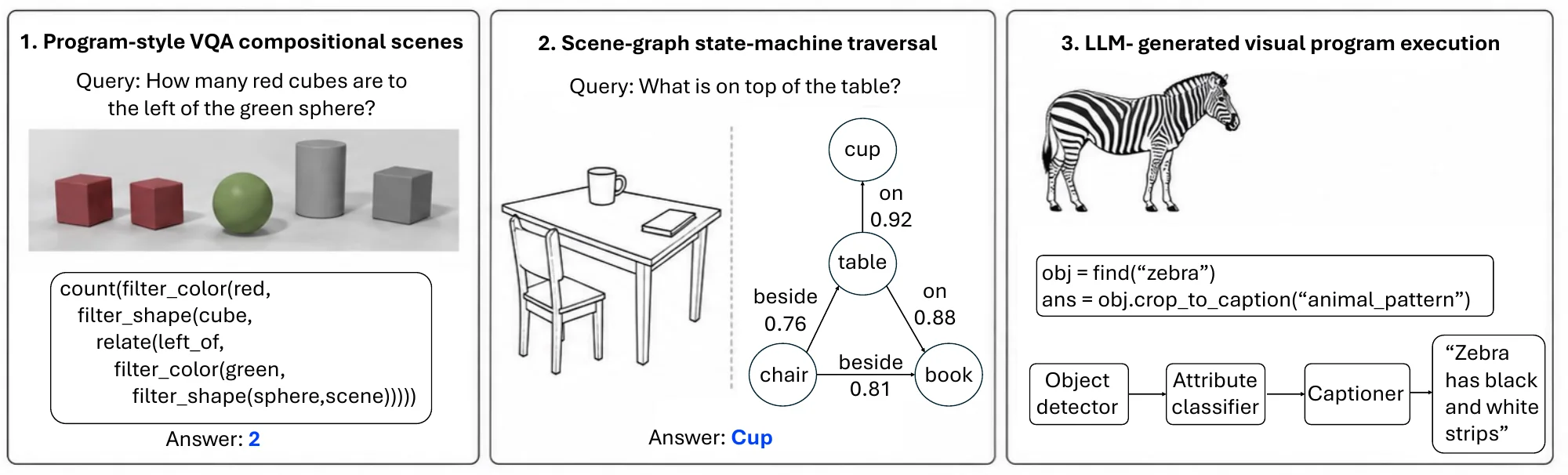
7.2.2.1Task Definition#
Given a visual observation (a single image or a set of views) and a query or goal , the system constructs an intermediate structure and executes it,
| (7.20) |
where may be a program layout , a recurrent sequence of reasoning states, a scene graph with a finite-state traversal over its nodes, or a code trace that calls external tools, and the executor realizes through neural modules, symbolic operators, graph transitions, or tool calls. The output may be an answer, a localized region, a predicted relation, or an action. The defining property is therefore not a specific program syntax but the presence of an inspectable that mediates between perception and prediction, which is what makes the reasoning path explicit and controllable.
7.2.2.2Methodology#
The four families in Figure 7.10 differ in how much structure they expose, enough to make reasoning inspectable and compositional, but not so rigid that a perception error, a parser error, or a missing primitive causes deterministic failure. Each exposes a different facet of space: recurrent architectures a temporal trace of attentional focus, scene-graph methods object-centric relations, program-based methods named operations such as filtering, relating, counting, and comparing, and LLM-generated programs tool-call traces that combine detection, segmentation, localization, and external knowledge.
Structured Recurrent Reasoning Architectures. This family imposes a step-wise reasoning structure in the architecture itself, so the model is fully differentiable and trained end-to-end from input–output pairs while still exposing a step-by-step trace. The Memory, Attention, and Composition (MAC) network [1360] chains recurrent cells, each of which attends to the question to choose the operation for the current step (control unit), extracts the relevant visual information by spatial attention guided by that control signal (read unit), and integrates it into a reasoning state passed to the next cell (write unit); the attention maps of successive read units provide a transparent trace of where the model is looking, without a rigid symbolic program. MAC is thus a boundary case: explicit at the level of reasoning dynamics, implicit at the level of spatial representation, since the operations run over dense feature maps rather than named objects or relations. Because the spatial logic stays in the learned weights, it is prone to statistical shortcuts (if “red spheres” co-occur with “cubes” in training, the model may learn that correlation rather than “left of”), and soft attention maps are often diffuse, so “to the left” bleeds into irrelevant regions in cluttered scenes.
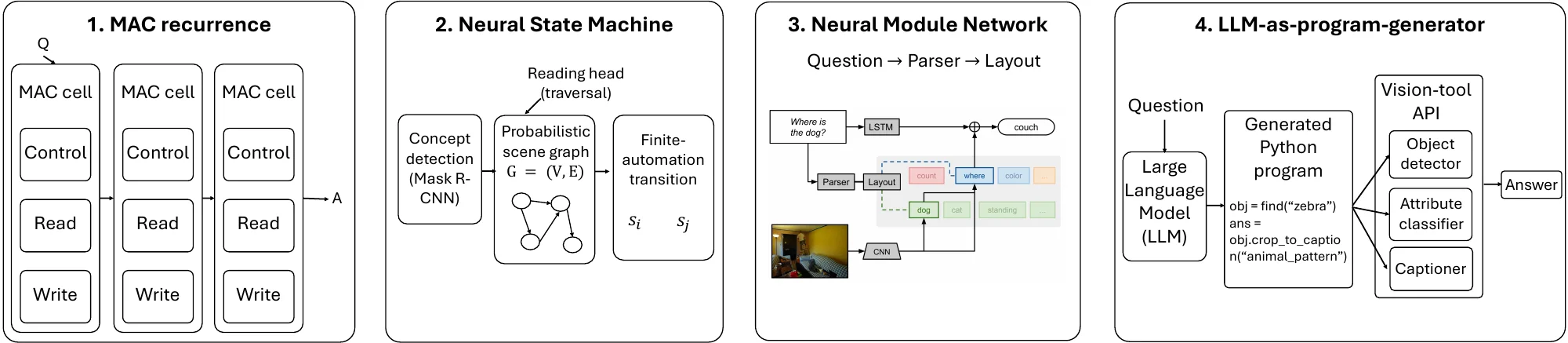
Structured Scene Representations. A related line strengthens the structural prior on the reasoning substrate. Where MAC reasons over a soft grid of features, the Neural State Machine (NSM) [1361] reasons over a discrete semantic scene graph and simulates a finite automaton over it: a concept-detection module (Mask R-CNN) identifies entities, each node is initialized with semantic properties over a learned concept vocabulary, each edge carries a distribution over spatial and semantic relation types (left of, behind, on top of, holding), and the query is answered by sequentially traversing nodes along valid transitions. More broadly, scene graphs act as a generic structured substrate: a downstream reasoner can traverse the graph as a hard environment (the NSM stance), attend over it as a soft relational prior, or search it for graph-based question answering, in each case obtaining an inspectable cut-point between perception and reasoning. The price is that reasoning quality becomes tightly coupled to object detection, attribute grounding, and relation prediction, a dependency we return to in the challenges.
Modular and Program-Based Reasoning. A third family translates the query itself into an executable program, and its members differ mainly in the nature of the executor. The Neural Module Network (NMN) [1362] is the canonical neural-executor instance: an external semantic parser converts a question such as “What color is the llama?” into a layout, e.g., , classify[color](attend[llama]), whose slots are instantiated by distinct learnable modules (attention, re-attention, classification, combination, measurement) trained jointly to maximize the likelihood of the gold answer. Because NMN relies on an off-the-shelf parser, IEP [1363] replaces it with a sequence-to-sequence program generator that emits the program as a sequence of functions, trained jointly with the execution modules via REINFORCE [1367] or by maximizing answer likelihood over a distribution of programs. Moving further toward symbols, Neuro-Symbolic VQA (NS-VQA) [1364] adopts a symbolic executor: a scene parser turns the image into a symbolic table, after which the program reduces to deterministic functional operators, yielding fully interpretable execution at the cost of a near-perfect-perception assumption. The Neuro-Symbolic Concept Learner (NS-CL) [347] occupies the middle ground with a quasi-symbolic executor: a neural perception module produces object-centric representations and a semantic parser emits symbolic programs, but the executor relaxes discrete operations such as filtering and relating into differentiable ones, so the whole system trains end-to-end from answers alone.
LLM-Generated Visual Programs. The most active recent extension lets a large language model emit the program directly, replacing the seq2seq parser of IEP or the hand-crafted parser of NMN with a tool-based executor. ViperGPT [1131] and VisProg [1365] pair a frozen LLM with a Python-style API of vision tools (detectors, captioners, attribute classifiers) that the generated code invokes, making the approach compositional and zero-shot without per-task training. Code-as-Policies [1366] pushes the same program-synthesis paradigm into embodied control, treating the LLM-emitted program as a closed-loop policy over perception and actuation primitives; it is included here as an embodied extension of the paradigm rather than as a VQA method. The interpretability gain is real, since the emitted code is human-readable, but these systems re-inherit the brittleness of the underlying LLM (hallucinated API calls, ungrounded tool routing) as a failure mode the earlier hand-coded DSLs were designed to avoid.
Unifying View: Parser, Representation, Executor, and Supervision. The four families are points in a shared design space with four axes. The parser that maps a query to structure may be hand-built (NMN), learned end-to-end (IEP, NS-CL), or a frozen LLM (ViperGPT, VisProg); the representation over which reasoning runs may be a dense feature map (MAC), an object-centric scene graph (NSM, and the scene-graph-generation literature [798] supervised at scale by Visual Genome [796]), or a symbolic scene table (NS-VQA); the executor may be neural, symbolic, quasi-symbolic, or a code interpreter; and the supervision may be answer-only, program-supervised, or, in tool-based systems, augmented with execution traces and tool feedback. The inspectable structure between perception and answer is the common thread: it provides a natural cut-point at which symbolic and learned components can be swapped without retraining the rest of the stack, and the same four axes reappear in the foundation-model reasoners of §7.3.
Beyond VQA: 3D, Temporal, and Embodied Extensions. The same design pattern extends beyond static images: referring-expression grounding has been lifted from 2D images to 3D scenes [374], where object-centric and spatial-relation graphs supply the substrate for reasoning about support, containment, proximity, and navigability, and in video and embodied settings the intermediate structure becomes a temporal scene graph or a task plan that links perception to action (§7.3, Part IV). These extensions also expose the central limitation of current explicit methods: most available program primitives and graph predicates are still designed for static 2D relations, whereas viewpoint change, object permanence, physical interaction, and multi-step navigation need 3D, temporal, and causal operators.
7.2.2.3Benchmarks and Performance#
The CLEVR family [1358] of §7.2.1 is the canonical testbed here as well, with the added property that each question is generated alongside a ground-truth functional program, which gives both program-supervised and answer-only training signals; MAC, IEP, NS-CL, and NS-VQA all converge to the high-90s on it, making it attractive but saturated. GQA [839] is the dominant open-domain benchmark: it pairs natural-image scenes with compositional questions whose ground-truth scene graphs (from Visual Genome [796]) make scene-graph-based reasoners directly applicable, and its out-of-distribution splits expose the systematic-generalization gap hidden by saturated CLEVR scores. VQA v2 [1359] remains the reference point for visual-program systems such as ViperGPT and VisProg, which are evaluated zero-shot on GQA and VQA v2. Referring-expression grounding benchmarks (RefCOCO and RefCOCO+ [1082], RefCOCOg [1083], and the earlier ReferItGame [1088]) are equally relevant, since they test whether a system can bind spatial language (“the object left of / behind / next to …”) to a localized region even when the output is a box or mask rather than an answer. Embodied program-as-policy systems such as Code-as-Policies are evaluated by task success in robotic or simulated manipulation environments and should not be compared against VQA accuracy. Table 7.1 collects the headline numbers.
| Method | Structure exposed | Supervision | CLEVR | GQA |
| RN [1349] | none (pairwise latent) | answers | 95.5 | – |
| FiLM [1355] | none (feature modulation) | answers | 97.7 | – |
| MAC [1360] | recurrent control / read / write | answers | 98.9 | 54.1 |
| IEP [1363] | generated program, neural executor | programs (700k) answers | 96.9 | – |
| NS-CL [347] | program, quasi-symbolic executor | answers (curriculum) | 98.9 | – |
| NS-VQA [1364] | program, symbolic executor | scene tables 270 programs | 99.8 | – |
| NSM [1361] | probabilistic scene graph, automaton | answers | – | 63.2 |
| ViperGPT [1131] | LLM-generated code, tool executor | none (zero-shot) | – | 48.1 |
| VisProg [1365] | LLM-generated code, tool executor | none (zero-shot) | – | 50.5 |
7.2.2.4Challenges and Trends#
Exposing programs, graphs, state transitions, or tool calls buys interpretability but creates new failure modes, and the numbers above locate them. The first bottleneck is parsing: if a question is mapped to the wrong program or traversal path, even a correct executor produces the wrong answer. The second is symbol grounding and underspecification: spatial predicates such as Left, Behind, Near, or Between depend on viewpoint, scale, object extent, and task context, so many spatial queries do not determine a unique program, a single deterministic DSL operator is often too rigid, and new predicates demand manual re-engineering of the executor. The third is error propagation: mistakes by the detector, scene parser, relation classifier, or program generator are inherited by the executor and can cause deterministic failure, which is why NSM reaches 63% on GQA while the same family saturates CLEVR; on natural images the bottleneck has moved from reasoning execution to perception, scene-graph construction, language grounding, and long-tail relation coverage. A fourth, more structural tension is the differentiability–interpretability trade-off: the more symbolic the executor, the more auditable but the harder to train end-to-end; the more differentiable, the more robust but the less transparent. Because the value of explicit structure lies in the intermediate trace, evaluation should move beyond final-answer accuracy to whether the parsed program is faithful to the query, whether graph edges correspond to real relations, whether tool calls are necessary and grounded, and whether the execution trace actually supports the answer.
Most explicit systems also reason over static 2D layouts or object graphs rather than 3D geometry, temporal dynamics, or physical causality: they can answer whether is left of , but rarely simulate how a scene changes under motion, contact, containment, support, or occlusion, which is exactly the mental-simulation capacity human-level spatial reasoning requires. LLM-generated programs widen the scope by replacing fixed parsers with flexible code generation, trading a small accuracy gap on saturated benchmarks for zero-shot generality across VQA, grounding, and knowledge-grounded VQA, but they add hallucinated tool calls, invalid APIs, ungrounded intermediate variables, and the absence of a verifiable execution loop. The emerging direction is therefore not a return to purely symbolic reasoning but verifiable hybrid systems, in which learned perception produces object-centric representations, structured programs or graphs provide an inspectable scaffold, and neural or tool-based executors absorb the variability of real visual inputs, the direction of §7.3 and §7.4.
7.2.3Geometry-aware Neural Spatial Reasoning#
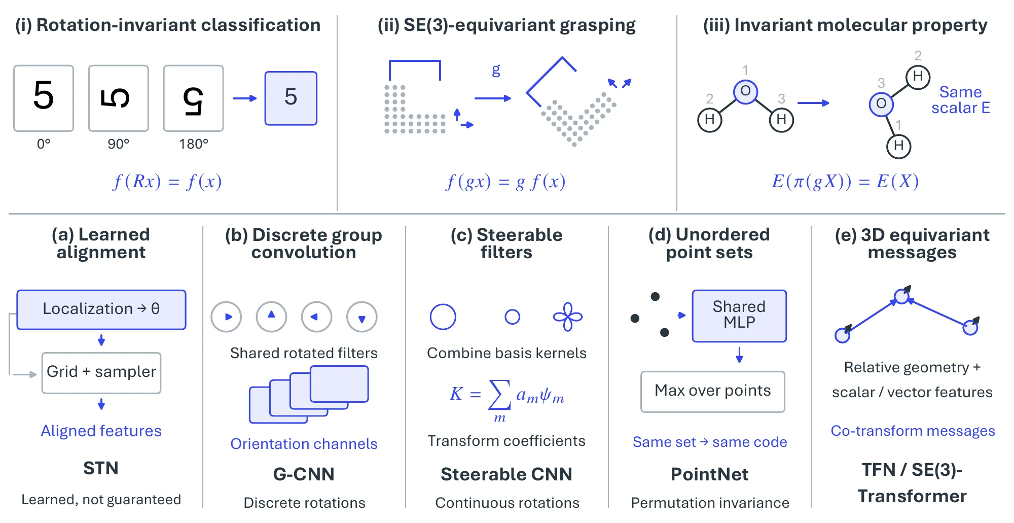
Where the implicit and explicit methods above learn spatial relationships from data, geometry-aware approaches build the relevant symmetries into the network itself: an object rotated, translated, or re-indexed keeps its identity, and the architecture is constructed so that this holds by design rather than being learned from many transformed examples. The gain is sample efficiency and robustness under the chosen transformations; the cost is that the symmetry group has to be chosen in advance. Figure 7.11 pairs three symmetry-driven task settings with the method families that supply the matching inductive bias.
7.2.3.1Task Definition#
The input lives in a space with a known geometric structure (a 2D image, a 3D point cloud, a molecular graph), optionally with a query , and the network is designed to respect a chosen group of transformations: translations for standard CNNs, rotations SO(3), rigid motions SE(3), or permutations of set elements. Its output is either invariant or equivariant to the action of .
Invariance vs. equivariance. An invariant representation stays fixed under the group action, , and deliberately discards pose; an equivariant representation co-transforms with the input, , where is the representation of the group action on the feature space, and thereby preserves it. In either case geometric consistency is a native constraint that the architecture guarantees by construction.
7.2.3.2Methodology#
Invariance is the right target when the output should not depend on orientation or position (classification), equivariance when pose and relative arrangement are the point (manipulation, keypoints, instance segmentation, molecular modeling); the layers below realize each.
Invariance by Pooling and Augmentation. The baseline strategies work without changing the architecture. Augmenting the training set with rotated, flipped, or scaled copies pushes a standard CNN toward assigning the same label to all variants, but buys only an approximate invariance and requires examples of every transformation to be tolerated; global average pooling [1371] at the end of a feature extractor discards the “where” of each feature and keeps only its presence, which is the main reason classification CNNs are robust to translation. Neither guarantees invariance to anything beyond translation.
Active Alignment with Spatial Transformer Networks. Rather than ignoring transformations, a Spatial Transformer Network (STN) [1368] learns to undo them: a small localization network regresses the parameters of an affine transformation that it predicts will bring the object into a canonical pose, a grid generator turns these parameters into a sampling grid, and a differentiable sampler produces the rectified feature map, so the localization network is trained by backpropagation from the task loss alone. The module can be inserted at any point in a network and acts as learned attentional alignment, normalizing a region of interest for the layers downstream; the invariance it provides is learned, not guaranteed.
Permutation Invariance over Point Sets. A separate symmetry arises when the input is an unordered set rather than a grid: the model must be invariant to the ordering of its elements. DeepSets [1372] shows that any permutation-invariant function over a set can be written as for suitable and , encode each element independently, sum, then decode, which turns set-level invariance from an ad-hoc choice into a constructive recipe and makes explicit which aggregators preserve invariance and which silently break it; the same framework yields permutation-equivariant layers for per-element outputs (per-point labels, per-atom properties). PointNet [132] is the canonical instance on raw point clouds, a shared multilayer perceptron per point followed by symmetric max pooling, and PointNet++ [270] adds locality by repeatedly grouping points within a metric ball and applying the same shared-MLP-plus-pool pattern at multiple scales. Permutation invariance comes for free in this family; rigid-motion invariance does not, which is the gap the equivariant methods below address.
From Translation to Group Equivariance. A standard convolution is translation-equivariant (shifting the image shifts the feature map) but not rotation-equivariant: rotating the input changes the feature map unpredictably. Group equivariant convolutions (G-CNNs) [1357] generalize the operation to a larger discrete group such as the four planar rotations: a single filter is rotated into a set of transformed copies, all are correlated with the input, and the feature map gains an orientation dimension, so a feature that reads “edge at ” becomes “edge at ” at the corresponding location when the input rotates by . Equivariance is therefore not learned but imposed, layer by layer.
Steerable Filters and Equivariance in Every Layer. Steerable CNNs [1369] replace the group-indexed filter copies by filters expressed in a steerable basis, so that the response at a transformed orientation follows by linear combination of basis responses rather than by explicit rotation; the general E(2) framework [1373] extends this to continuous rotations and reflections with circular-harmonic bases under one configurable interface, and library efforts such as e3nn [1374] do the same for E(3) / SE(3). Full equivariance also requires that pooling, nonlinearities, and normalization respect the group: a standard ReLU applied to the components of a geometric vector breaks it (activations are therefore applied to invariant quantities such as the vector norm), and channel-wise batch normalization breaks the coupling between channels, which motivates equivariant normalization [1375]. The guarantee is only as strong as its weakest layer; one non-equivariant operation anywhere in the stack silently undoes the symmetry the rest preserve.
Equivariant Attention and Continuous SE(3) Symmetries. A more recent line lifts the treatment from convolutions to attention, with queries, keys, and values that transform predictably under a chosen Lie group. The SE(3)-Transformer [379] is the canonical instance, building each attention layer from tensor-field representations so that rotating the input scene rotates the whole stack of outputs consistently; Tensor Field Networks [1370] use the same machinery without an attention head and have been especially influential in molecular modeling, where SE(3) equivariance is a problem constraint rather than an optional bias. Both parameterize the kernel as a combination of spherical-harmonic basis functions, which is computationally heavy, so a parallel line pursues lighter equivariance: E()-equivariant graph networks (EGNN) [1376] achieve E()-equivariant message passing from relative distances and coordinate updates alone, and Vector Neurons [380] lift scalar point-cloud features to 3D vectors, obtaining SO(3) equivariance as a drop-in primitive, each trading representational richness for scalability. With the libraries above, trying equivariance on a new task now costs about as much engineering as a convolutional baseline; the choice of group still has to be made by the designer.
7.2.3.3Benchmarks#
Benchmarks in this area are constructed to expose behavior under symmetry transformations. MNIST-rot is the standard 2D testbed, separating methods that learn rotation robustness through augmentation from those that build it in; ModelNet40 [1377] evaluates point-cloud classification under three protocols, aligned training and test (z/z), training with azimuthal rotations and testing under arbitrary SO(3) rotations (z/SO(3)), and arbitrary rotations in both (SO(3)/SO(3)), which is where augmentation, STN-style alignment, and PointNet’s permutation-invariant pooling are separated from genuine rotation handling; ScanObjectNN [1378] adds real scan noise and occlusion. For equivariance as a hard constraint, QM9 [1379] (small-molecule property prediction) and interatomic-potential tasks are the reference, where the SE(3)-equivariant models NequIP [1380] and MACE [1381] set the current points for data efficiency and accuracy. Table 7.2 reports the two ladders on which the method families can be compared directly.
| Method | MNIST-rot err. | z/z | z/SO(3) | SO(3)/SO(3) |
| Plain CNN (Z2CNN) [1357] | 5.03 | – | – | – |
| P4CNN (G-CNN) [1357] | 2.28 | – | – | – |
| E(2)-steerable CNN [1373] | 0.68 | – | – | – |
| PointNet [132] | – | 85.9 | 19.6 | 74.7 |
| PointNet++ [270] | – | 91.8 | 28.4 | 85.0 |
| VN-PointNet [380] | – | 77.5 | 77.5 | 77.2 |
| VN-DGCNN [380] | – | 89.5 | 89.5 | 90.2 |
7.2.3.4Challenges and Trends#
The most fundamental difficulty is choosing the symmetry group: invariance to a group that is too large (SO(3) when only SO(2) is task-relevant) destroys discriminative information, invariance to one too small leaves the model brittle to the symmetries the task actually exhibits, and the trade-off has no purely data-driven solution [1357, 1369]. Cost scales with the group: classical equivariant architectures index filters by group elements, so parameters and memory grow with the size of the chosen group, limiting how freely reflections, multi-scale rotations, or higher-order tensor representations can be included [1373]. The assumption of exact symmetry is also brittle: point clouds with self-occlusion, partial-view RGB, and noisy LiDAR scans do not realize an SO(3)-orbit, so an architecture that is mathematically equivariant can still fail when the input violates the assumed structure. Table 7.2 shows where the two targets diverge: on 2D classification both hand-coded invariance and learned equivariance saturate, so data efficiency rather than accuracy becomes the discriminating axis, while on ModelNet40 the invariance-only PointNet family collapses under unseen rotations and the equivariant family holds its accuracy, because the task requires geometric information to be preserved, not discarded. Finally, hard equivariance sits uneasily with the attention-based representations that dominate the rest of the stack (§7.2.1, §7.2.2, vision–language pretraining): self-attention is permutation-equivariant but not rotation-equivariant, and bolting an equivariant layer onto an attention pipeline often degrades the inductive bias that motivated the choice.
Equivariant attention is the main compromise on offer, and frame averaging [1382] moves in the opposite direction, turning any off-the-shelf backbone into an invariant or equivariant one by symmetrizing its outputs over a small input-dependent set of group frames, which decouples the choice of symmetry from the choice of architecture and sidesteps the parameter cost of group-indexed filters. These threads are pulling geometry-aware reasoning back toward the rest of the chapter: vision–language and vision–language–action models attach equivariant heads where 3D pose and geometric consistency matter, as in grasp policies and pose-conditioned generation, and primitives first devised for object classification are finding second lives in world models, embodied control, and 3D generation.
7.2.4Differentiable Optimization Layers for Spatial Reasoning#
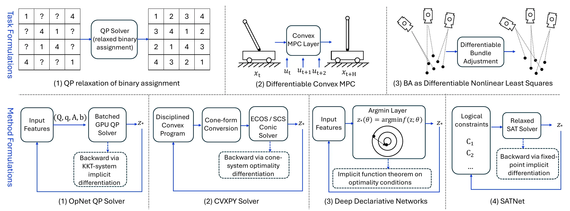
Where the three preceding subsections put structure into the learned representation, differentiable optimization layers put it into the computation: selected feed-forward operations are replaced by the solution of a constrained optimization problem, so that hard logical, geometric, or physical constraints are enforced inside the forward pass while the whole system stays end-to-end differentiable [1383]. In spatial reasoning this is how a network enforces distances, collision avoidance, or alignment, or solves a sub-problem such as pose estimation, within a learnable pipeline. Figure 7.12 previews the representative tasks (top row) and the method families (bottom row).
7.2.4.1Task Definition#
Given an input parameter vector produced by the preceding layers, a differentiable optimization layer computes
| (7.21) |
where is an objective function, denote inequality and equality constraints, and is a feasible domain. The forward pass computes the optimal solution , while the backward pass relies on implicit differentiation of the optimality conditions to obtain ; the layer is declarative, in that the model specifies what to solve rather than how to compute it. Under this view, QP solvers [1384], convex optimization layers [1387], differentiable geometry solvers [95], and differentiable logic program solvers [1385, 1391] are all instantiations of the same layer, tailored to different domains of spatial or symbolic reasoning.
7.2.4.2Methodology#
QP and Convex Optimization Layers. Amos and Kolter [1384] introduced OptNet, which treats the solution of a quadratic program as a layer: the forward pass solves
subject to affine constraints whose matrices can depend on previous network outputs, and the backward pass differentiates the KKT optimality conditions exactly, with a custom GPU interior-point solver that handles many small QPs in parallel and reuses its factorization for the backward pass. OptNet learned to solve Sudoku from data where conventional architectures could not, which showed that implicit layers can handle discrete or constrained reasoning problems. Agrawal et al. [1387] generalized the idea to any disciplined convex program: CVXPY Layers [1388] canonicalize the problem into conic form, solve it, and differentiate through the cone program’s optimality conditions, so a constrained least-squares, a constrained logistic regression, or a robot-motion-limit constraint can be inserted as a layer without deriving gradients by hand.
Implicit Differentiation. All of these layers share one mechanism. Rather than unrolling an iterative solver, one differentiates the closed-form optimality (KKT) conditions, which for a convex program comprise primal feasibility, dual feasibility, complementarity, and stationarity [1392]; differentiating this system and solving one linear system yields exactly, without back-propagating through solver iterations. Where OptNet hand-codes this backward pass, Deep Declarative Networks [1389] apply automatic differentiation to the KKT system itself. The same principle extends to root-finding, fixed-point, and equilibrium layers via the implicit function theorem; deep equilibrium models [1393] treat an entire weight-tied network as a single fixed-point layer differentiated this way, and differentiable physics engines and planners propagate gradients through the equilibrium or optimum conditions of a physical system.
Differentiable Geometry Solvers. A subclass is tailored to geometric problems that are themselves argmin problems, typically minimizing a reprojection error: camera pose from 2D–3D correspondences, bundle adjustment, inverse kinematics. Campbell et al. [1390] introduced a differentiable blind PnP solver that estimates 3D pose as a layer; Teed and Deng [95] built a differentiable bundle-adjustment module into a SLAM system, solving for camera poses and 3D points by iterative optimization while letting gradients flow; EPro-PnP [744] recasts PnP as a probabilistic layer with a learnable distribution over poses; and Theseus [1394] provides a reusable library for differentiable nonlinear least squares (Gauss–Newton, Levenberg–Marquardt) that underlies bundle adjustment, pose-graph optimization, and inverse kinematics. These layers keep the domain-specific optimizer but make it differentiable, so the whole vision or robotics system trains end-to-end while the geometry stays correct and constrained, for instance so that estimated object poses agree across views; Gould et al. [1389] refer to such constructs as declarative nodes and demonstrate them on visual Sudoku and robust geometry estimation.
Differentiable Logic Layers. Beyond continuous optimization, the same construction extends to symbolic reasoning. SATNet [1385] integrates a differentiable satisfiability solver as a layer: the forward pass solves a relaxed SAT problem (a quadratic unconstrained binary optimization) to produce assignments consistent with logical constraints, and the backward pass differentiates implicitly through the solver’s fixed-point conditions; Shindo et al. [1391] extend differentiable logic programs to abstract visual reasoning benchmarks such as Raven’s Progressive Matrices. These layers belong to the same class of constraint-based implicit modules as the QP and convex layers, specialized to combinatorial and relational dependencies.
7.2.4.3Benchmarks#
Differentiable optimization layers have been validated across symbolic, geometric, and control settings. Sudoku [1384, 1385] and its visual variant [1383] test whether a layer models constraint satisfaction and propagates gradients through discrete reasoning; Raven’s Progressive Matrices (RPM / I-RAVEN) [1391] test whether differentiable logic captures relational structure in visual analogy puzzles; cart-pole, inverted-pendulum, and reaching tasks in MuJoCo and OpenAI Gym [1387] test whether differentiable MPC [1386] or convex layers improve control while enforcing physical feasibility; and maze navigation and obstacle avoidance test QP-based collision-avoidance layers by whether the agent reaches its target without violating safety constraints. Evaluation combines task metrics with criteria specific to the embedded solver: geometric accuracy (translation / rotation error in pose estimation, trajectory or map error for a bundle-adjustment layer), task success rate (puzzles solved, feasible plans produced) together with the count or magnitude of violated constraints and, for physics-informed layers, residual energy or momentum drift, and solver cost and gradient stability (forward / backward runtime, iterations to converge, and sensitivity of training to approximate versus exact implicit gradients). Table 7.3 lists the representative layers by solver type.
| Method | Year | Solver / layer type | Task / benchmark |
| OptNet [1384] | 2017 | QP layer, KKT implicit diff. | Sudoku from data |
| Differentiable MPC [1386] | 2018 | convex MPC layer | planning / control |
| CVXPY Layers [1387] | 2019 | disciplined convex / cone layer | control, geometry |
| SATNet [1385] | 2019 | differentiable MAXSAT relaxation | visual Sudoku |
| Deep Declarative Nets [1389] | 2021 | implicit-function-theorem nodes | robust geometry, Sudoku |
| DROID-SLAM [95] | 2021 | differentiable bundle adjustment | monocular / stereo SLAM |
| Theseus [1394] | 2022 | differentiable nonlinear least squares | pose-graph / BA / IK |
| EPro-PnP [744] | 2022 | probabilistic PnP layer | monocular 6-DoF pose |
7.2.4.4Challenges and Trends#
Solving an optimization problem inside a layer is more expensive than a convolution or a matrix product, and the forward pass becomes the bottleneck as problem size grows, which is exactly the regime of SLAM, bundle adjustment, and motion planning. OptNet’s batched GPU solver shows how problem structure buys tractability for many small problems, but global route planning or large-scale 3D reconstruction still overwhelms existing solvers, forcing approximate solves, warm starts, or hierarchical decomposition to keep each optimization manageable.
Gradient stability is the second difficulty. If the solution is non-unique or depends discontinuously on the input, as at boundary optima, at active-set changes in a linear program, or in the presence of discrete variables, the implicit gradient is unstable or undefined; strict convexity guarantees a well-defined Jacobian, and real problems frequently violate it. Entropy smoothing, small regularizers, and perturbation methods restore usable gradients in many cases, and in others the backward pass has to be designed by hand.
The third is physical consistency. An optimization layer enforces only the constraints it is given: if the formulation omits a friction constraint in a contact model, the network exploits the gap and converges to implausible solutions, and because the layer sits inside a trainable system, the surrounding network can learn to feed it inputs that satisfy the constraints superficially while violating their intended meaning. The benefits of interpretability and correctness therefore depend on the optimization model reflecting the real dynamics, which in practice means careful constraint modeling, additional penalties, or iterative refinement of the solver design; current work refines solvers, numerical stability, and integration with deep-learning frameworks toward layers that are both theoretically grounded and deployable in spatial systems.
7.2.5Reinforcement Learning with Spatial Inductive Biases#
Where the previous four subsections constrain the learned representation, reinforcement learning shifts the locus of structure to the action-conditioned setting, in which an agent must reason about spatial relationships as a consequence of its own behavior over a long horizon. Many spatial tasks, such as navigation, exploration, manipulation, and embodied interaction, cannot be reduced to static perception or single-step prediction; they require reasoning about how actions transform the agent’s position, orientation, and relations to surrounding objects over time, under geometric constraints, partial observability, and delayed reward. Generic RL policies built on unstructured function approximators struggle to generalize across unseen layouts, so a growing body of work introduces spatial inductive biases, explicit planning iterations, map-like latent representations, differentiable search operators, or relational state abstractions, that constrain the hypothesis space of policies or value functions to reflect the compositional and geometric structure of spatial decision-making.
7.2.5.1Task Definition#
At each step the agent receives an observation from the environment (RGB / RGB-D frames, egocentric maps, point clouds, language goals) together with its action history , chooses an action from a continuous control space or a discrete set , and receives a scalar reward . The policy or value function is parameterized with a spatial structural prior (a differentiable planning module, a learned map or belief representation, a relational or graph encoder, an equivariant policy head),
| (7.22) |
so that shapes which policies and value functions the agent considers in the first place, not only how it generalizes after the fact; the optimization itself remains a standard RL objective (Bellman, policy gradient, actor–critic, or preference-based).
7.2.5.2Methodology#
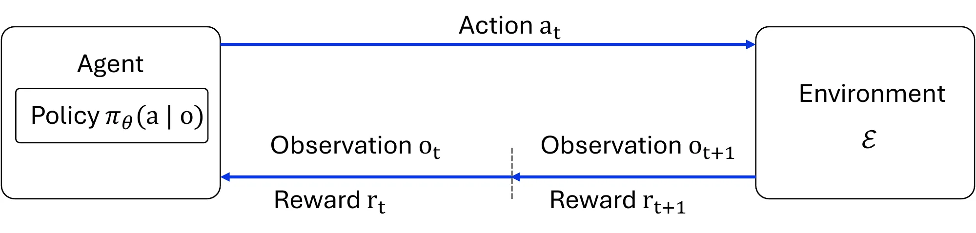
Figure 7.13 shows the loop every method below shares: the agent observes, acts, receives a reward and a new state, and updates its policy to maximize long-term return. Learning a good policy requires balancing exploration of untried actions against exploitation of the actions currently believed best, the exploration–exploitation trade-off that underlies all of RL. The subsections that follow walk through the optimization backbones in the order the field developed them, value-based, policy-based, actor–critic, PPO, and the recent preference-based and group-relative objectives, and note at each step where spatial structure enters.
Value-Based RL. Value-based methods learn a value function that estimates the expected cumulative return of acting under a policy . The optimal state-action value function is
| (7.23) |
where is the discount factor, and it satisfies the Bellman equation: if the optimal values of the next state are known for every action , the best action now is the one that maximizes ,
| (7.24) |
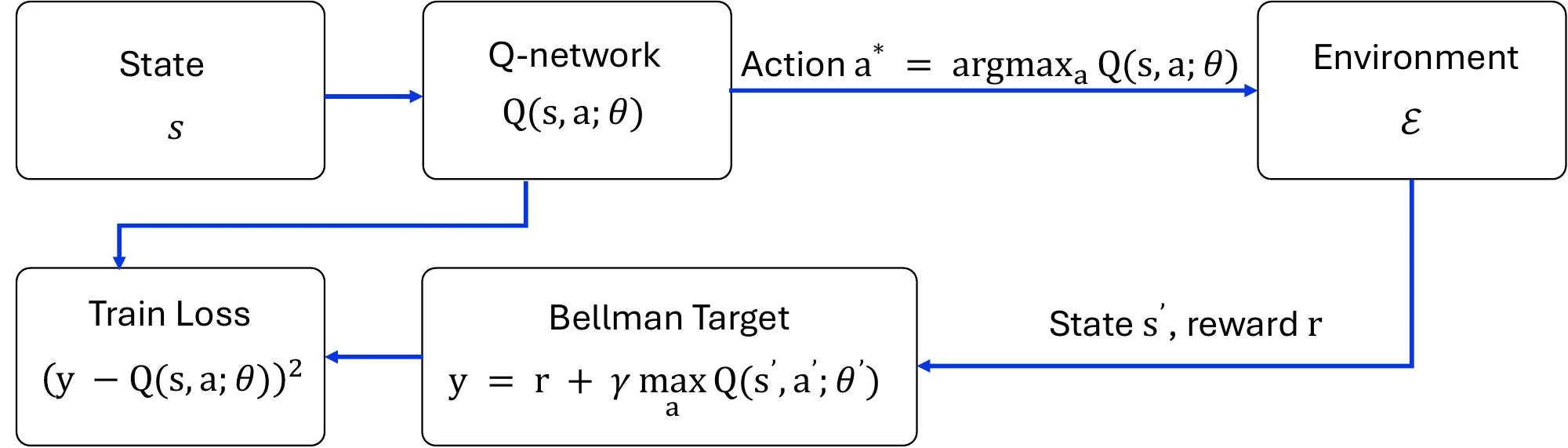
Iterating this identity as an update, , converges to , but a table of values indexed by every state is useless in high-dimensional observation spaces, so a function approximator is learned instead, a neural network in the deep-RL setting (a Q-network). Training minimizes a sequence of regression losses whose target is the bootstrapped Bellman estimate,
| (7.25) |
with computed from the previous parameters , held fixed, and the distribution of visited state–action pairs; the greedy policy then follows from the learned values.
Deep Q-networks (DQN) [1395] made this scale to high-dimensional observations with experience replay and a slowly updated target network; their convergence is analyzed theoretically by Fan et al. [1396], and Figure 7.14 shows the resulting workflow. Beyond control, value-based RL drives active visual perception: Caicedo and Lazebnik [1397] cast object localization as a sequential decision process in which a Q-network iteratively transforms an attention window until it tightly bounds the target, turning detection into a learned spatial search policy, a formulation since applied to active detection, visual search, and region selection for fine-grained recognition, where the agent learns where to look rather than scanning exhaustively. In spatial domains the limitation of vanilla DQN is that any planning behavior must be learned implicitly from data, which generalizes poorly to novel layouts, so several works embed planning structure in the value estimate itself. Value Iteration Networks (VIN) [1398] unroll Bellman updates as convolutions over a spatial grid, a differentiable approximation of value iteration; Gated Path Planning Networks (GPPN) [1399] replace the recurrence with gated units to improve optimization stability and long-range dependencies; and under partial observability QMDP-Net [1400] integrates belief updates and approximate POMDP planning (QMDP) [1401] into one differentiable network. In each case the learned value function is constrained to follow spatially structured dynamic programming rather than arbitrary function approximation.
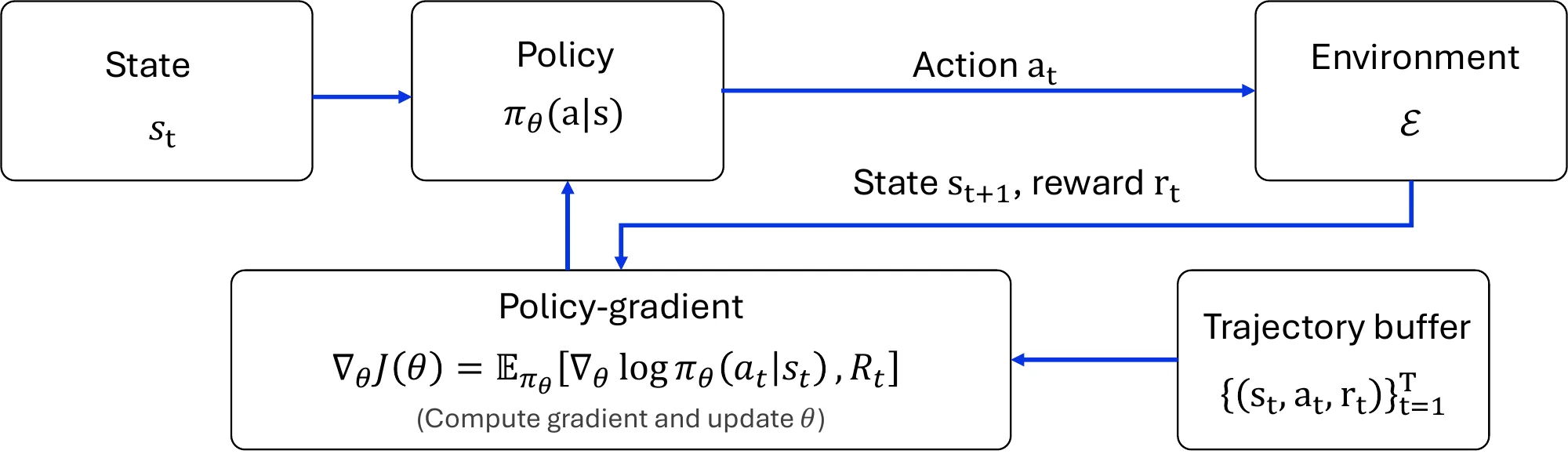
Policy-Based RL. Policy-based methods [1367, 1402] parameterize a policy directly and maximize expected return,
| (7.26) |
by gradient ascent on
| (7.27) |
where is the return from time-step (Figure 7.15). Optimizing action distributions directly suits spatial decision problems in which exploration and long-horizon credit assignment are central [1403], and policy gradients train embodied agents to actively gather visual evidence: Embodied Question Answering [1404] optimizes a navigation policy so that the agent moves to vantage points from which it can answer questions about a 3D scene. The spatial competence, however, comes from the architecture rather than the objective; policy-gradient agents generalize across layouts when the policy carries a learned map [1405], a grounded spatial representation [1406], memory, or a relational encoder [1407].
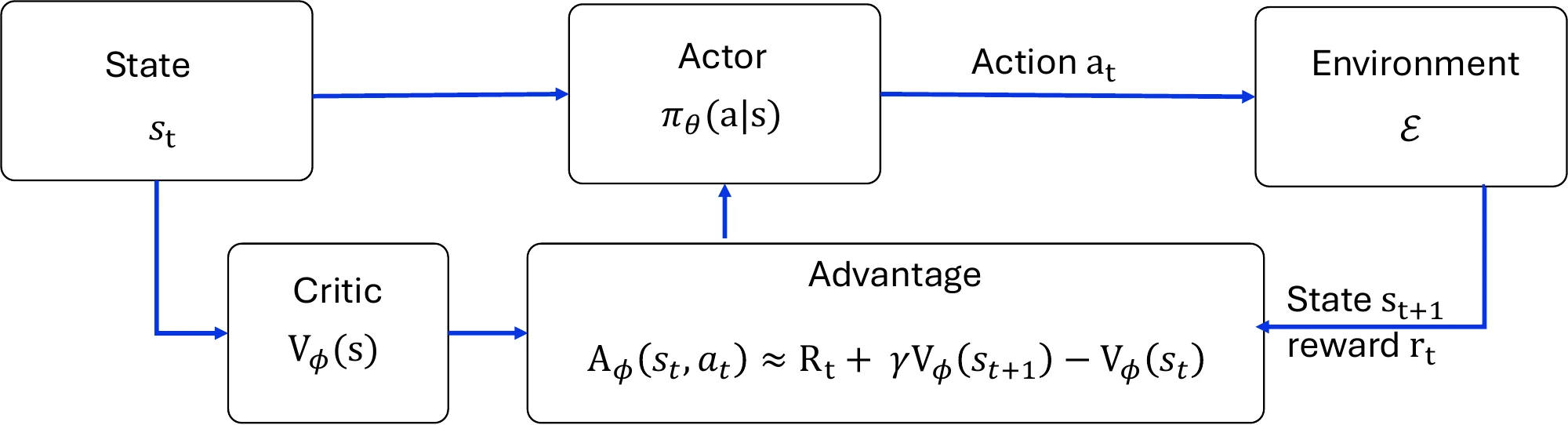
Actor-Critic RL. Actor–critic methods [1408] combine the two by jointly learning a policy (the actor, which controls behavior) and a value function (the critic, which scores the actions taken), as in Figure 7.16. The critic provides a low-variance estimate of the advantage,
| (7.28) |
or, when a Q-function is learned as well, , and the advantage replaces the raw return in the policy-gradient update. The asynchronous advantage actor-critic (A3C) [1409] made this stable and scalable and became a standard backbone for embodied navigation and spatial control: target-driven visual navigation [1410] conditions an A3C agent on an image of the goal and reaches semantically specified targets in unseen indoor scenes, and Neural SLAM [1411] gives an A3C agent a differentiable map memory. The separation between actor and critic matches the structure of spatial tasks, with the actor responsible for geometry-aware decisions and the critic supplying global, long-horizon value signals, which is why actor–critic methods dominate navigation benchmarks that require memory, planning, and partial observability [1412].
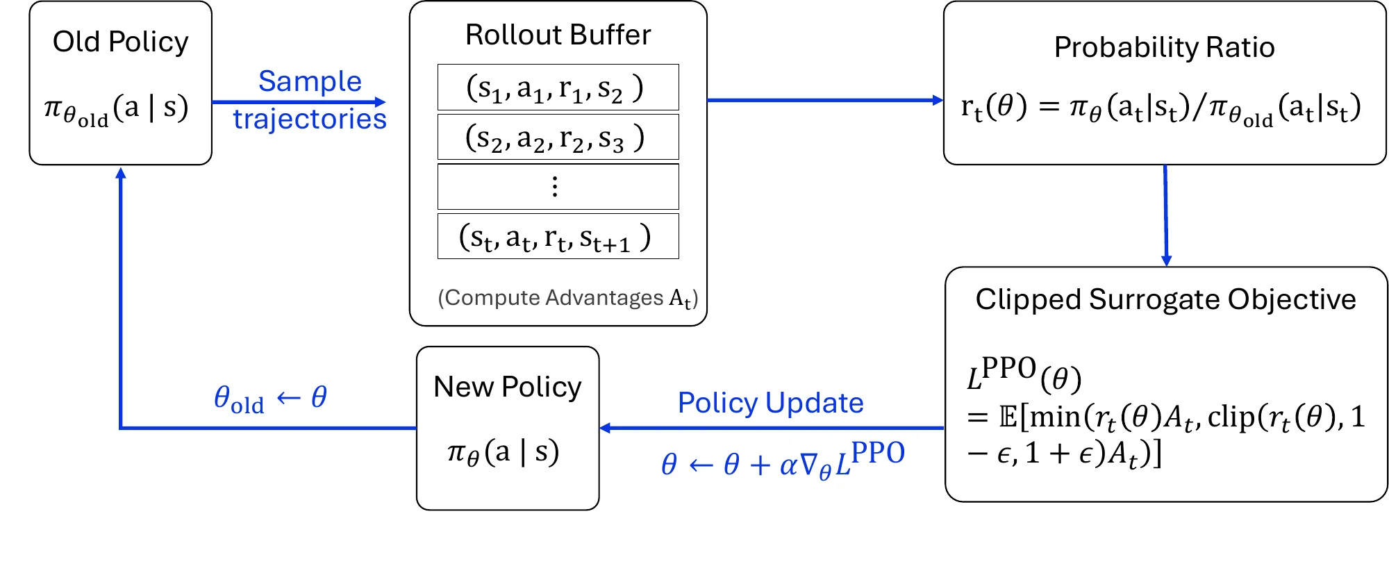
PPO-Style Policy Optimization. Proximal Policy Optimization (PPO) [1413] is an actor–critic algorithm that stabilizes training by constraining each policy update through a clipped surrogate objective,
| (7.29) |
where is the probability ratio between the new and old policies (Figure 7.17). Its robustness and sample efficiency made PPO the de facto backbone for training agents in large-scale photorealistic 3D simulators such as Gibson [93] and Matterport3D [340], and in manipulation suites such as panda-gym1. Scaled to 2.5 billion frames with DD-PPO [1414], it essentially solves PointGoal navigation on Habitat (99.7% success and 0.97 SPL on Gibson validation), and the same backbone underpins vision-and-language navigation [1415], object-goal navigation [1416], audio-visual navigation [46], and planning over uncertain topological maps [1417].
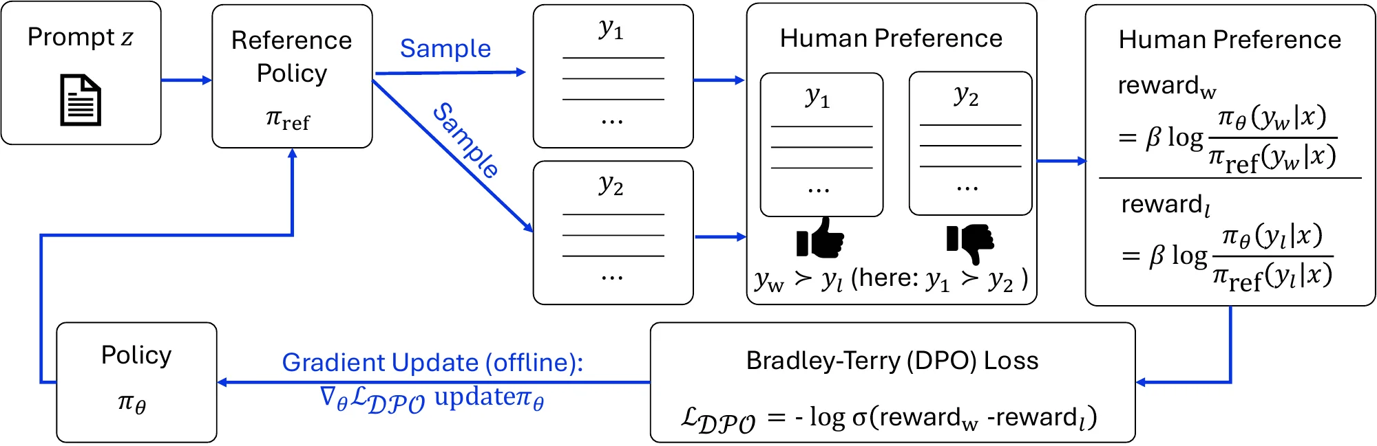
Preference-Based Policy Optimization (DPO). Preference-based learning replaces the reward signal with comparisons. Direct Preference Optimization (DPO) [1418] learns a policy from preference pairs without an explicit reward model or online rollouts (Figure 7.18): for two completions of an input , a labeler marks the preferred one, , and by expressing the implied reward of a Bradley–Terry preference model [1419] through the optimal policy itself, DPO collapses the reward-learning-then-RL pipeline into a single maximum-likelihood objective on :
| (7.30) |
where is a fixed reference policy and controls the deviation from it. Developed for language-model alignment, DPO applies to spatial reasoning whenever supervision takes the form of trajectory preferences, plan rankings, or human judgments of spatial behavior [1420, 1421, 1422], which arise naturally in navigation, manipulation, and interactive tasks where dense rewards are hard to specify.
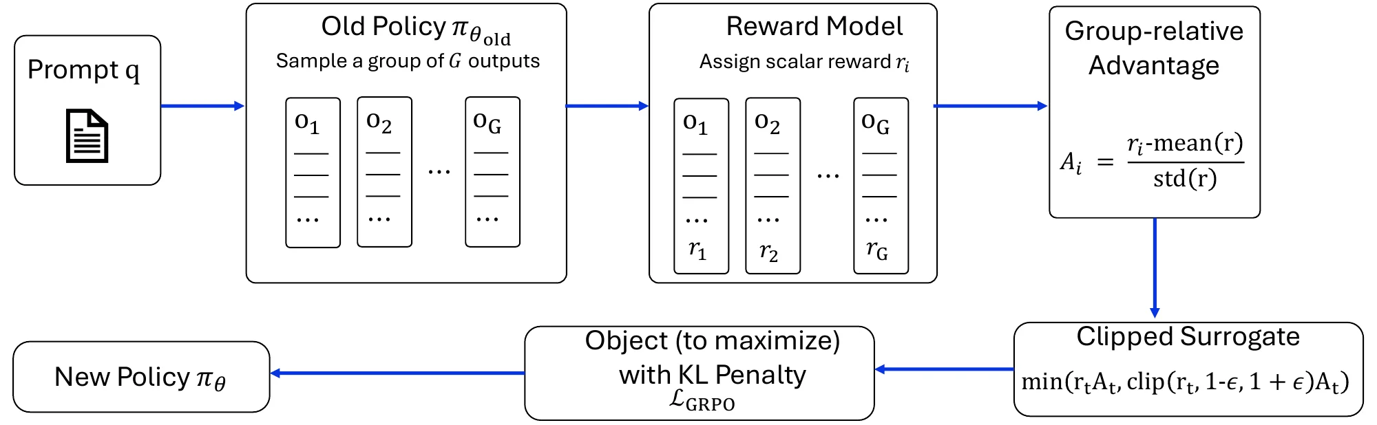
Group-Based Policy Optimization (GRPO). Group Relative Policy Optimization (GRPO) [1423] removes the learned critic and replaces it with a group-relative baseline computed from multiple sampled trajectories (Figure 7.19). For each question , it samples a group of outputs from the old policy and optimizes by maximizing
| (7.31) |
where and are hyperparameters and the advantage is computed from the rewards that a reward model assigns to the group, normalized within the group only:
| (7.32) |
Eliminating the value network reduces memory and stabilizes training. Although explored first for language models, the formulation transfers to spatial decision-making wherever several candidate plans or trajectories can be scored against one another, and it has become the standard recipe for reinforcement fine-tuning of spatial vision–language models on visual reasoning, navigation, multi-step assembly, and video spatial reasoning [1424, 1425, 1426, 1427].
Architectural Spatial Inductive Biases. The backbones above are domain-agnostic; what makes a policy spatial is the prior in its architecture, and three families recur across the examples already met. Map-based representations give the agent an explicit allocentric memory: cognitive maps [1405] and Neural Map [1428] write observations into a spatially indexed latent grid, while Neural SLAM [1411] and Active Neural SLAM [1429] couple differentiable mapping with a hierarchical exploration policy. Differentiable planning modules embed dynamic programming in the network, as in the VIN / GPPN / QMDP-Net line discussed under value-based RL, or learn a value-equivalent model and plan by lookahead search, as in MuZero [148]. Relational abstractions replace flat feature maps with object- or graph-structured state, letting attention or message passing capture relations that transfer across layouts [1407]. In each case the RL objective is unchanged; the spatial competence comes from the prior, which is why these architectures generalize across geometries where unstructured policies overfit.
7.2.5.3Benchmarks#
Two complementary benchmark families shape the empirical landscape. Embodied navigation and exploration benchmarks stress long-horizon planning under partial observability in photorealistic 3D scenes: Habitat [94] is the dominant platform, paired with real-world scans from Matterport3D [340] and Gibson [93] for large, scene-diverse PointGoal and ObjectGoal navigation that exercises geometry-aware exploration and cross-scene generalization; SoundSpaces [46] adds audio-visual cues as a multimodal test of spatial state estimation; and SOON [1430] extends vision-and-language navigation to scenario-oriented object goals in unseen environments. Symbolic and relational benchmarks test whether structured priors yield combinatorial and compositional generalization: PDDLGym2 builds Gym environments from PDDL domains with relational observations and actions, and lightweight gridworld suites such as MiniGrid3 support controlled evaluation of planning, memory, and compositional generalization; the differentiable planners (VIN, GPPN, QMDP-Net) are evaluated on procedurally generated gridworld mazes and POMDPs of increasing size, where the question is whether the architectural prior generalizes to unseen layouts rather than memorizing training mazes. Across both families the choice of RL algorithm matters less than the choice of prior: PPO has converged as the standard optimizer for embodied navigation, and differences between agents mostly reflect the map, planning module, or relational encoder on the policy, while on gridworld benchmarks the methods that embed planning structure consistently dominate unstructured DQN, with the largest gains where the task is most planning-shaped.
7.2.5.4Challenges and Trends#
Sample inefficiency comes first. Spatial tasks involve long horizons, sparse rewards, and combinatorial state spaces, so naïve exploration is prohibitively expensive; architectural priors such as learned maps, planning modules, and relational representations improve efficiency [1398, 1402], but current RL systems still need orders of magnitude more interaction than humans or classical planners to acquire robust spatial competence.
Generalization and transfer come second. Many agents perform well in their training environments and degrade sharply in unseen layouts, novel geometries, or altered dynamics, which suggests that much of the learned behavior rests on superficial correlations rather than abstract spatial structure; structured state representations, world models, and modular policy design [1403, 1405] help, but how to enforce spatial invariances and compositional generalization in RL in a principled way remains open.
Reward specification is the third. Spatial tasks often lack dense, well-defined rewards, especially when success depends on long-term plan quality, safety, or efficiency rather than immediate outcomes. Preference-based methods such as DPO [1418] and group-relative objectives such as GRPO [1423] learn from comparative feedback instead, at the price of reward-model bias, preference inconsistency, and the difficulty of aligning learned preferences with the true task objective in complex spatial domains.
The directions that follow from these three are hybrid methods that integrate learning with explicit planning or search [1398, 1400], structure-aware representations (object-centric, relational, graph-based) that scale spatial reasoning beyond grid-based and navigation-centric benchmarks [1407], and evaluation protocols that weight out-of-distribution generalization, robustness to environmental variation, and reasoning quality over performance on fixed benchmarks.
7.2.6Multi-agent Spatial Reasoning#
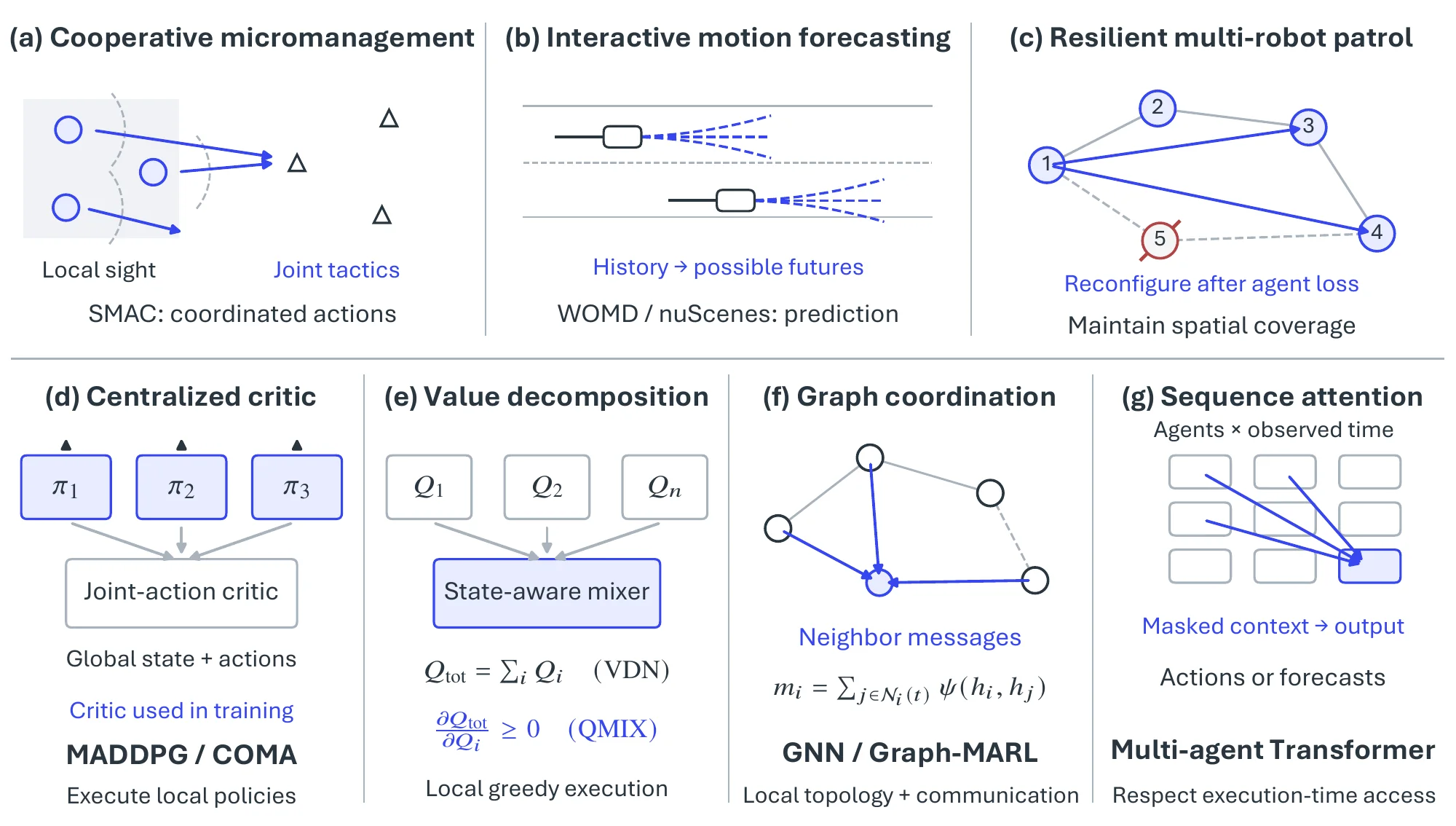
Where the previous five subsections study a single learning agent, multi-agent spatial reasoning (MASR) moves to the joint regime: multiple embodied or abstract agents perceive, communicate, and act within a shared environment to accomplish cooperative or competitive goals, and the structural prior now governs decentralized decisions over a shared spatial state. MASR links low-level sensorimotor streams (proprioception, occupancy grids, trajectories) to relational decision processes (joint planning, role assignment, coalition formation); its core problem is credit assignment and coordination under spatial constraints, that is, how agents with partial, decentralized observations reason over nearby entities, infer latent intent, and synthesize actions that produce coherent team-level behavior. Deep learning has moved the field from rule-driven coordination to end-to-end policies that integrate perception, communication, and control under partial observability and non-stationarity [1431, 1432, 1433], with autonomous driving and interactive motion forecasting over road geometry (WOMD [218], nuScenes [445]), multi-robot exploration, formation control, and patrol under attrition [1434], and real-time strategy and team-sports simulation [1435, 1436] as its representative domains. We stress at the outset that the canonical algorithms surveyed below (VDN, QMIX, COMA, MADDPG) are themselves spatially agnostic: they solve a generic cooperative Dec-POMDP and see geometry only through the environment and the reward. Explicit spatial structure enters chiefly through the benchmarks and through the graph-based family, where the interaction graph makes neighborhood relations a first-class part of the policy.
7.2.6.1Task Definition#
We cast cooperative multi-agent spatial reasoning as a graph-structured Dec-POMDP
| (7.33) |
with a (possibly time-varying) interaction graph derived from state (e.g., , proximity or visibility) or estimated locally. At time , agent receives a partial egocentric observation (RGB-D, LiDAR, occupancy, kinematics) and optional neighbor messages ; we treat as the input available to agent , with any bandwidth cost included in . Agents act with decentralized, history-dependent policies
| (7.34) |
the joint policy factorizes as , and the objective is
| (7.35) |
In predictive variants, auxiliary heads output multi-agent forecasts or spatial fields with confidences for planning or losses; these are not environment actions. Settings differ along two further axes: online methods act in streaming settings under tight latency, whereas offline methods learn from logged interaction data (e.g., , driving datasets) with batch updates and conservative behavior constraints; and centralized training with decentralized execution (CTDE) exploits global state to train joint value functions or critics while enforcing decentralized policies at test time [1432, 1433], whereas fully decentralized learning never accesses global state, trading sample efficiency for deployability.
7.2.6.2Methodology#
Figure 7.20 summarizes the tasks above and the method families discussed below.
Classical Paradigms. Before learning, coordination relied on potential fields, formation keeping via graph Laplacians, and optimal multi-agent pathfinding with conflict-based search [1228], treated in §7.1.3; these methods offer strong guarantees but struggle with perception noise, combinatorial scaling, and model mismatch in open worlds.
CTDE and Value Decomposition. Two lines made CTDE work. Centralized critics resolve credit assignment and non-stationarity while keeping execution decentralized: COMA uses a counterfactual baseline computed by a centralized critic for decentralized actors [1432], and MADDPG extends deterministic policy gradients with agent-specific centralized critics [1431]. Value factorization instead decomposes the joint value: VDN sums per-agent utilities to approximate for cooperative tasks [1437], and QMIX generalizes the sum to a monotonic mixing network that preserves individual-global argmax consistency with more representational capacity [1433]. These approaches made MARL scalable on SMAC [1435], where the value-decomposition line dominated the early cooperative leaderboard while the centralized-critic methods anchored other regimes (MADDPG on the particle environments, COMA on StarCraft micromanagement); the monotonic constraint and homogeneous-role assumptions limit expressivity, as the challenges below detail.
Graph Neural Networks for Coordination. Graph-based MARL encodes agents as nodes and interactions as edges, and message passing or attention over the neighborhood learns role-specialized coordination [1438]; this family improves sample efficiency and robustness under topology changes and communication limits, and MAGEC [1434] shows resilience to agent attrition and communication disturbance in multi-robot patrol by combining GNN encoders with PPO-style multi-agent optimization. Graph MARL targets a different axis from the leaderboard methods, robustness to topology disturbances rather than headline return, which exposes a gap between coordination-quality benchmarks (SMAC, MPE) and deployment-quality ones (multi-robot patrol, driving forecasting on WOMD and nuScenes) that standardized suites still under-represent.
Sequence Models and Transformers. Casting MARL as sequence modeling applies attention over multi-entity, multi-horizon contexts: the Multi-Agent Transformer [1439] maps the sequence of agents’ observations to a sequence of actions with an encoder–decoder, using the multi-agent advantage decomposition to turn joint policy search into sequential decisions with linear complexity in the number of agents. Transformer controllers, often hybridized with graph layers, address long-range temporal and relational dependencies, unify perception and control, and support offline RL through trajectory modeling; learned memory alleviates partial observability, while quadratic attention and credit assignment over long horizons remain open.
7.2.6.3Benchmarks#
Benchmarks span two regimes: simulation suites that stress cooperation, partial observability, and communication learning under controlled physics and reward shaping, and real-world multi-agent trajectory datasets that test interactive prediction and motion forecasting at deployment scale. Table 7.4 summarizes the most widely used resources.
| Dataset / Suite | Year | Scale | Action/Task Space |
| SMAC [1435] | 2019 | 22+ micro scenarios | Discrete, decentralized |
| Multi-Agent Particle Env. (MPE) [1431] | 2017 | 10+ 2D templates | Continuous/discrete |
| GRF [1436] | 2020 | Dozens of tasks / full-game | Continuous/discrete |
| nuScenes [445] | 2020 | 1,000 scenes 20 s @ 2 Hz | Trajectory prediction |
| WOMD [218] | 2021 | scenes 20 s @ 10 Hz | Trajectory prediction |
| Neural MMO [1440, 1441] | 2020 | Persistent worlds; agents | Long-horizon survival |
Evaluation depends on whether the setting is control or prediction. Control is scored by mean episodic return , success or win rate, time-to-goal, collision and rule-violation rates, fairness or load-balancing indices for cooperative logistics, and communication overhead; prediction and planning are scored by spatial accuracy, from displacement errors over the forecast horizon (minADE, minFDE, miss rate on WOMD and nuScenes) to intersection-over-union between predicted and ground-truth occupied regions or trajectory tubes.
7.2.6.4Challenges and Trends#
Multi-agent spatial reasoning faces structural difficulties that distinguish it from the single-agent settings of §7.2.1–§7.2.5, organized here along four axes within the classical multi-agent paradigm.
Credit Assignment under Partial Observability and Long Horizons. The decentralized-execution constraint of the Dec-POMDP forces each agent to act on its own history alone, so relating a local action to a delayed team-level reward across a horizon produces an irreducibly noisy policy gradient. Counterfactual baselines such as COMA [1432] marginalize over alternative actions of agent while holding the rest of fixed and reduce gradient variance substantially, but they still rely on a centralized critic that, at scale, becomes a moving target for itself. Value decomposition (VDN, QMIX) [1437, 1433] side-steps the centralized critic by factorizing across agents, yet the monotonicity constraint that guarantees decentralized argmax consistency cannot represent strictly non-monotonic cooperation games, a representational ceiling made explicit by the later non-monotonic factorizations QTRAN, weighted QMIX, and QPLEX, and visible on cooperative matrix games and SMAC’s hardest scenarios [1442, 1443, 1444, 1435]. Under sparse reward shaping, policies trained against these signals tend to chase short-term spatial cues (“move toward the closest enemy”, “follow the nearest teammate”) rather than team-level objectives.
Scaling Laws of Joint Reasoning and Communication. Sequence-model multi-agent Transformers and dense graph message passing both incur complexity in the number of agents, plus additional quadratic terms across temporal contexts, which collides with the real-time latency budgets of multi-robot [1434] and autonomous-driving deployments [218, 445]. Sparse, learned interaction graphs are the natural mitigation, but they introduce their own credit-assignment difficulty: the edges are themselves part of the learned policy, and gradients flowing through hard edge selection are biased or high-variance. Communication bandwidth is a related gap: in the formulation above any message should carry a cost that appears in , but the standard simulators (SMAC [1435], MPE [1431], GRF [1436]) idealize communication as free and noiseless, leaving little benchmark surface against which to push bandwidth-aware coordination.
Non-stationarity, Heterogeneous Roles, and Partner Generalization. Even in fully cooperative settings, intra-team policies co-evolve, so from the perspective of any single agent the environment is non-stationary [1431], the failure mode the centralized-critic family of MADDPG / COMA [1431, 1432] was introduced to address. The problem sharpens when teammates are heterogeneous, may drop out (the patrol-with-attrition setting of MAGEC [1434]), or are drawn from an unseen partner distribution at evaluation time, the zero-shot coordination problem. Persistent open-world simulators such as Neural MMO [1440, 1441] push along this axis with procedurally generated maps and long-horizon survival, but standardized protocols for partner generalization and role specialization remain immature compared with the single-agent supervised benchmarks of §7.2.1 and §7.2.3.
Ambiguous Spatial Semantics and Sim-to-Real Transfer. The egocentric observations that drive decentralized policies are partial and noisy: occluded teammates, uncertain affordances, and depth-discontinuity-induced map errors distort both prediction and control. Driving benchmarks such as WOMD [218] and nuScenes [445] expose the prediction side of this gap, but the closed-loop control side (whether the same forecasts survive when an agent acts on its own predictions) is comparatively under-evaluated. The sim-to-real gap on multi-robot systems is wider still: perception noise and actuation latency interact non-linearly with the coordination signal in ways that simulators rarely model, and resilience under realistic communication disturbance and agent attrition has only recently received first-class benchmark coverage [1434].
Three routes follow from these axes. Topology-aware sparse interaction (learned edges, hierarchical groupings, or attention masks parameterized by ) preserves long-range coordination while scaling sub-quadratically, with the GNN+PPO patrol architecture of MAGEC [1434] as an early instantiation and graph encoders combined with sequence-model attention over short temporal windows as the natural next step. The monotonicity ceiling of VDN / QMIX [1437, 1433] can be relaxed by attention-weighted mixers, weighted projection schemes, or dueling-style decompositions that keep individual-global argmax consistency while admitting non-monotonic cooperation, so that COMA-style counterfactual credit assignment [1432] no longer depends on a joint-action critic that becomes the bottleneck. And explicit objectives for agent attrition and communication disturbance [1434], paired with failure-centric curricula and hooks for formal verification, move resilience from an emergent property of training to a first-class objective, decisive in safety-critical multi-robot and driving deployments [218, 445] where worst-case performance dominates the deployment decision; closed-loop evaluation suites that jointly report team return, safety, calibration, and latency are the missing measurement substrate, and the benchmarks for partner generalization, bandwidth-aware coordination, and sim-to-real transfer that would play the role SMAC and GRF played for CTDE are still under construction.