Everything to this point has described a single instant. Spatio-temporal perception adds the missing axis, asking not only where entities are but how they move, when events happen, and which identities persist. Its three concerns rise from the pixel through the object to the event: scene flow recovers dense, per-point motion between frames; object tracking maintains the identity of an entity as it moves through space and time; and temporal localization fixes when an action or event occurs along a sequence. Together they give the otherwise static perception of the preceding sections a temporal thread, the continuity on which motion understanding and long-horizon perception depend.
6.4.1Scene Flow Estimation#
Scene flow is the dense three-dimensional motion of every visible surface point between two instants: optical flow lifted out of the image plane and joined to the change in depth. The image-based pipelines surveyed here take stereo video, monocular video, or a multi-view sequence and produce per-pixel 3D motion; some refinement modules additionally consume estimated or measured depth. Dynamic scene reconstruction [299], motion-aware rendering [188], physical interaction modeling [680], and egocentric world understanding [681] all consume it.
6.4.1.1Task Definition#
Given consecutive frames and (optionally with a stereo partner or several views, and with intrinsics and relative poses when known), scene flow estimation returns a field that displaces the surface point imaged at pixel in frame to its position at , in camera or world coordinates. In the stereo setting this is equivalently a triple of disparity in both frames plus optical flow, which is how the KITTI benchmark represents and scores it. In image-only pipelines, structure and motion are inferred from appearance, parallax, and temporal correspondence. Geometry-aware refinement modules may instead take depth estimated upstream or measured by RGB-D sensors; point-cloud-only methods are outside the scope here.
6.4.1.2Methodology#
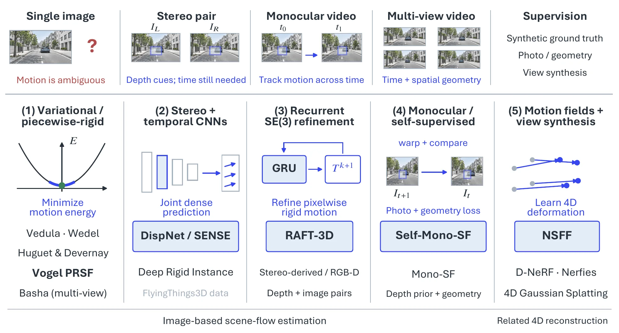
Methods differ along two axes: what they observe (stereo, the classical and still dominant setting; monocular video, the self-supervised frontier; multi-view rigs) and what supervises them (synthetic ground truth, photometric and geometric consistency, or view synthesis). Figure 6.21 groups them into five families along these axes.
Variational and energy-based methods. Vedula et al. [944] introduced the term and the problem: recover 3D structure and 3D motion jointly from a calibrated camera array. Huguet and Devernay [945] brought it to a single stereo pair, solving disparity and flow jointly in one variational energy; Wedel et al. [946] decoupled the two into a stereo stage and a flow stage, which made real-time estimation feasible; and Basha et al. [947] returned to multi-view input under a view-centered energy. The strongest classical formulation is the piecewise-rigid scene model of Vogel et al. [948] (PRSF/PRSM), which segments the scene into rigidly moving planar patches and was the leading entry on KITTI Scene Flow at the benchmark’s release.
End-to-end stereo and temporal CNNs. Mayer et al. [619] recast disparity and flow as supervised regression (DispNet, FlowNet) and released FlyingThings3D, Monkaa, and Driving, the synthetic corpora that made this training regime possible. SENSE [949] shares one encoder across disparity, optical flow, occlusion, and semantic heads; DRISF [950] keeps the piecewise-rigid prior of Vogel et al. but implements it as an instance-level decoder over learned features. Both surpassed the variational baselines on KITTI Scene Flow (Table 6.26), shifting the bottleneck from optimization to supervised data.
Recurrent geometric refinement. RAFT [255] introduced all-pairs correlation volumes with GRU-based iterative updates for 2D optical flow; RAFT-3D [951] uses image and depth pairs to iteratively refine a per-pixel SE(3) field with rigid-motion embeddings. Depth can be obtained from stereo or RGB-D input; it is an input to the refinement rather than necessarily inferred jointly from appearance. Its scene-flow results are included in Table 6.26.
Monocular and self-supervised methods. Mono-SF [952] was the first monocular entry on KITTI Scene Flow, resolving scale with a learned single-view depth prior. Self-Mono-SF [953] removes ground truth altogether, training depth, ego-motion, and 3D-motion heads on raw video through photometric and geometric consistency losses; the monocular depth priors of Section 6.2.1 and the ego-motion machinery of Section 6.2.4 are its two anchors. The same test-time-optimization idea applied to LiDAR point clouds (Neural Scene Flow Prior [954]) lies outside the image-based scope of this subsection.
Implicit-field and view-synthesis-coupled methods. A parallel line never targets scene flow as output but obtains a dense 4D motion field as a byproduct of dynamic view synthesis. Neural Scene Flow Fields [188] trains a dynamic NeRF together with an explicit scene-flow MLP; D-NeRF [187] represents motion as a deformation field into a canonical frame; Nerfies [299] extends this to casually captured monocular video; and 4D Gaussian Splatting [191] attaches time-parameterized motion to explicit Gaussian primitives. These methods are evaluated by rendering quality rather than by motion error, a split returned to under §Challenges.
6.4.1.3Datasets and Metrics#
Table 6.25 lists the image-based benchmarks. Synthetic sets provide dense, exact ground truth at scale (FlyingThings3D as the standard pretraining corpus; Sintel and Spring for film-grade motion, with Spring at HD resolution and super-resolved ground truth; TartanAir for environment diversity), while KITTI Scene Flow 2015 [955], built on the KITTI suite [173], is the only real-world benchmark and carries sparse LiDAR-derived labels on 200 training and 200 test scenes. LiDAR-based scene-flow splits of nuScenes [445], Waymo Open [446], and Argoverse 2 [661], and the event-camera flow of DSEC [941], serve the point-cloud and event communities and are not image-based benchmarks in the sense used here.
| Dataset | Year | Type | Input | Scale | Ground truth |
| KITTI Scene Flow 2015 [955] | 2015 | Real driving | Stereo video | 200 train / 200 test scenes | Sparse disparity (, ) + flow from LiDAR and CAD fits |
| FlyingThings3D / Monkaa / Driving [619] | 2016 | Synthetic | Stereo video | 25K / 8.6K / 4.4K frames | Dense disparity, flow, disparity change |
| MPI Sintel [956] | 2012 | Synthetic film | Stereo video | 1,041 train frames, 23 seq. | Dense flow, depth, disparity |
| Spring [957] | 2023 | Synthetic film | Stereo video | 6K frames, 47 seq., 19201080 | Dense stereo, flow, scene flow (super-resolved) |
| TartanAir [666] | 2020 | Synthetic | Stereo video | 1M frames, 30 environments | Dense depth, flow, pose; indoor and outdoor, weather |
KITTI scores scene flow in image space. A pixel’s disparity in frame (D1), its disparity in frame (D2), and its optical flow (Fl) are each counted as outliers when the error exceeds both 3 px and 5% of the ground-truth value, and a scene-flow outlier (SF) is any pixel that fails at least one of the three; the benchmark reports outlier percentages over all pixels and separately over background and foreground. Point-level evaluation on synthetic data instead uses the 3D end-point error
| (6.40) |
with and the predicted and true motion of point , together with accuracy ratios at fixed thresholds (the fraction of points with error below 0.05 m or 5%, and below 0.1 m or 10%) and an outlier ratio (error above 0.3 m or 10%), conventions inherited from point-cloud scene flow.
Table 6.26 collects KITTI Scene Flow 2015 test results for the explicit-output families. RAFT-3D more than halves the SF-all error of the best classical method (PRSM), and the foreground column, where rigidly moving vehicles meet non-rigid motion, is where the learned methods gain most. The monocular rows are a different regime: Mono-SF, with a learned depth prior, sits at 23% SF-all, and Self-Mono-SF without any ground truth at 49.5% (33.9% after fine-tuning), the price of giving up stereo. The implicit-field family has no row because it reports rendering quality (PSNR, LPIPS) on its own scene sets rather than motion error.
| Method | Family | D1-all | D2-all | Fl-all | SF-all |
| Stereo | |||||
| OSF [955] | Energy-based, rigid objects | 5.79 | 7.77 | 7.83 | 10.23 |
| PRSM [948] | Energy-based, piecewise rigid | 4.27 | 6.79 | 6.68 | 8.97 |
| SENSE [949] | Shared-encoder CNN | 2.22 | 5.89 | 7.64 | 9.55 |
| DRISF [950] | CNN + rigid instances | 2.55 | 4.04 | 4.73 | 6.31 |
| RAFT-3D [951] | Recurrent SE(3) refinement | 1.81 | 3.67 | 4.29 | 5.77 |
| Monocular | |||||
| Mono-SF [952] | Learned depth prior | 16.32 | 19.59 | 12.77 | 23.08 |
| Self-Mono-SF [953] | Self-supervised | 34.02 | 36.34 | 23.54 | 49.54 |
| Self-Mono-SF-ft [953] | Self-supervised, ft | 22.16 | 25.24 | 15.91 | 33.88 |
6.4.1.4Challenges#
The supervision landscape is lopsided. Every dense-ground-truth benchmark in Table 6.25 is synthetic and stereo, so monocular methods are scored only against KITTI’s sparse labels, and models pretrained on FlyingThings3D or Sintel still lose accuracy on real driving footage after fine-tuning, most visibly on foreground motion where synthetic random-object trajectories differ from vehicle kinematics. All current benchmarks also emphasize rigid or random-object motion; dense ground truth for non-rigid humans, hands, and animals does not exist at scale, which leaves the family of implicit-field methods that handle such motion best without a quantitative yardstick.
That yardstick problem is the second challenge. Explicit-output methods [948, 949, 951] are scored by KITTI’s outlier rates; implicit-field methods [188, 187, 191] by PSNR and LPIPS of rendered views. No protocol evaluates both on the same input, so the two paradigms are compared only qualitatively, and whether a motion field is good depends on whether scene flow is the end (the KITTI leaderboard) or a means (reconstruction, novel-view synthesis, physical reasoning). The cost profiles diverge as well: RAFT-3D needs several GRU iterations per frame, variational methods minutes per frame, and implicit fields minutes to hours per scene.
Foundation priors are reshaping the monocular line. Depth Anything [140] and DINOv2 [958] supply the per-pixel depth and semantic features that Self-Mono-SF had to learn from scratch, and SAM 2 [482] segmentation together with the object-pose estimators of Section 6.2.5 makes an object-centric formulation (a per-object SE(3) trajectory plus residual non-rigid motion) practical, a bridge to the tracking problem of Section 6.4.2. As implicit-field scene flow merges into 4D reconstruction, with 4D Gaussian Splatting [191] the early example, evaluation is likely to follow the downstream task rather than the KITTI leaderboard.
6.4.2Object Tracking#
Tracking localizes entities in every frame and associates the detections across frames so that each entity keeps one identity through the sequence. Where detection and segmentation describe a single instant, tracking yields trajectories, the representation that autonomous driving [959, 960], surveillance [961], AR/VR [220], and robotics [962] build on.
6.4.2.1Task Definition#
Given a frame sequence (a video, or RGB-D, LiDAR, or multi-view streams), a tracker returns a set of trajectories , each a time-indexed series of states with one identity held fixed over the sequence. The state is a bounding box in the basic setting and a segmentation mask, a 3D box, or a set of keypoints in the variants.
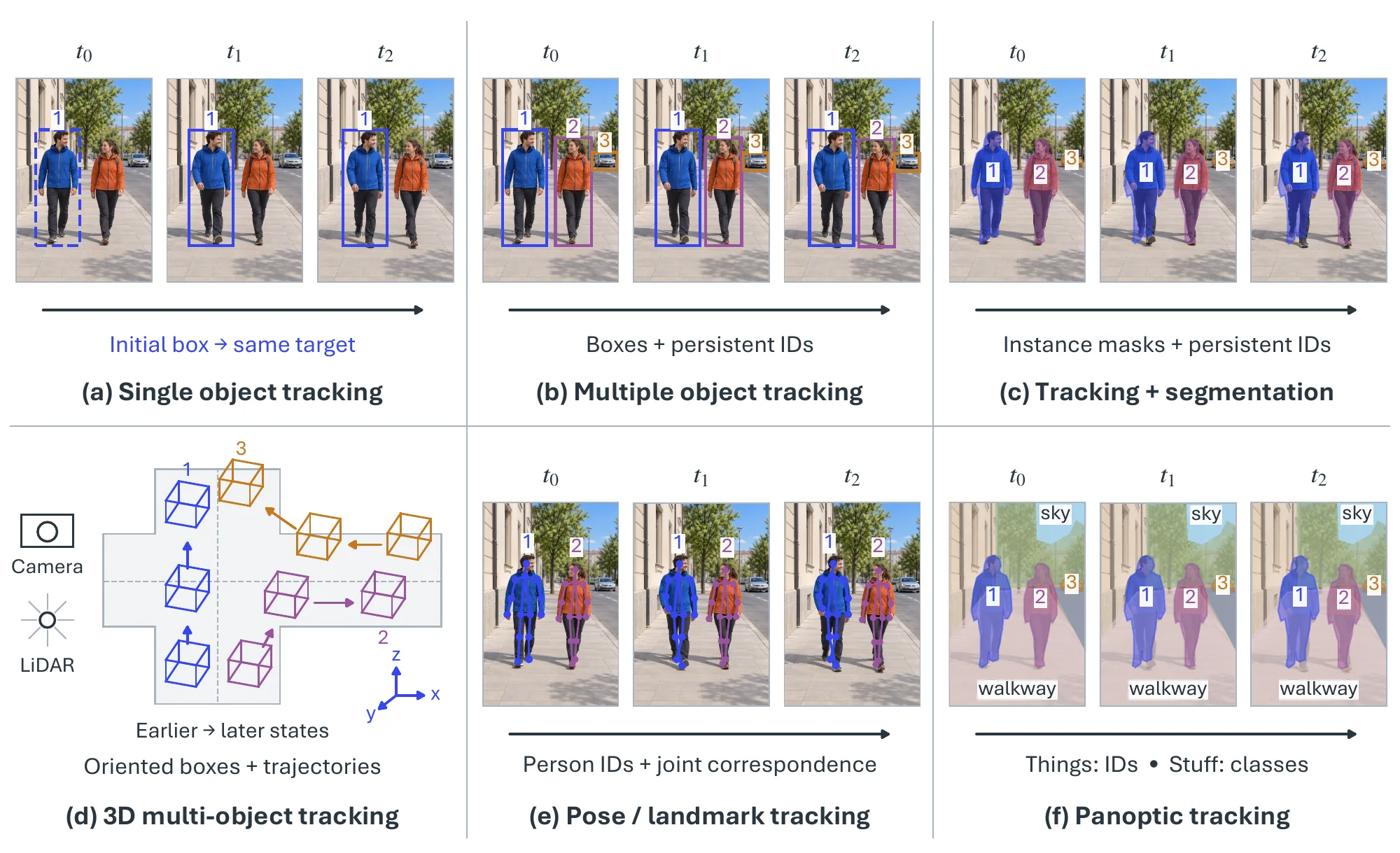
The variants, illustrated in Figure 6.22, differ in how the targets are specified and what state is tracked. Single object tracking (SOT) [963, 964] follows one target given its first-frame box; multiple object tracking (MOT) [965, 966, 711] tracks every instance of given categories, typically pedestrians and vehicles, under identity constraints; MOTS [967] and video object segmentation replace boxes with masks; 3D-MOT [968, 429, 445, 446] outputs world-coordinate 3D boxes from LiDAR, RGB-D, or multi-view input; pose tracking [549, 969, 970] and landmark tracking [971] follow skeletal joints or facial keypoints; and panoptic tracking combines pixel-level semantic classes for stuff with temporally consistent instance identities for things. Category-specific trackers for pedestrians [972], vehicles [973], or animals [974] specialize any of these.
6.4.2.2Methodology#
Figure 6.23 organizes the methods into four families around image-plane box and mask tracking (SOT, MOT, MOTS, VOS). Pose, landmark, and panoptic tracking reuse the same propagate-or-associate machinery with a different state representation and are covered at the benchmark level in Table 6.27.
Propagation-based methods. Because a target moves little between consecutive frames, its previous state is a strong prior for the current one, and the oldest tracking paradigm exploits this by predicting the next state from the current one and correcting it against the new frame. Correlation filters realize this in the frequency domain: MOSSE [975] learns a minimum-output-sum-of-squared-error filter from a single frame and updates it online at hundreds of frames per second; KCF [976] and MKCF [977] add kernelization and multi-scale search; ECO [978] adds factorized convolution operators, a compact generative sample model, and conservative updates. These trackers are fast enough for embedded use but drift under large appearance change and clutter. MDNet [979] answered with online discriminative learning, a shared CNN with per-sequence domain branches that separate target from background, at a high per-frame cost. Siamese trackers moved the representation learning offline: SiamFC [980] correlates a template embedding with the search-region embedding in one forward pass, and SiamRPN [981], ATOM [982], and DiMP [983] add region-proposal regression, IoU-prediction refinement, and a discriminatively learned prediction head. Transformer trackers then replaced correlation with attention: TransT [984] fuses template and search features with self- and cross-attention, STARK [985] predicts the box with an encoder–decoder that also carries temporal state, and OSTrack [986] joins feature extraction and relation modeling in a single stream over concatenated template and search tokens, the current baseline design.
Mask propagation applies the same idea at the pixel level for video object segmentation [987, 988], with memory of past frames replacing a single template. XMem [989] keeps multi-scale spatiotemporal memories that remain stable over videos of more than 10,000 frames; AOT [990] and DeAOT [991] encode object identities as tokens so that many objects propagate in one pass; and SAM 2 [482] adds a streaming memory to the Segment Anything Model [138], giving promptable tracking that transfers across VOS benchmarks.
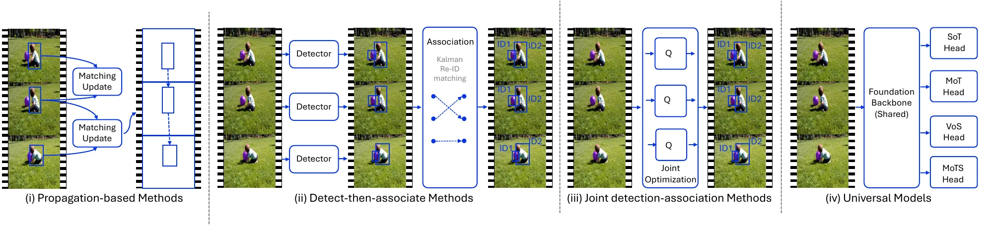
Detect-then-associate methods. The MOT standard pipeline detects objects in every frame and then solves an assignment problem between detections and existing tracks. SORT [992] predicts track positions with a Kalman filter [164] and matches by IoU with the Hungarian algorithm [993]; DeepSORT [994] adds an appearance embedding so that tracks survive occlusion. Track-RCNN [967], JDE [995], and FairMOT [996] train the re-identification embedding jointly with the detector; association remains a separate step, which keeps them in this family. All of these discard low-confidence detections, and since occluded targets are exactly those with low scores, trajectories fragment where they are hardest to keep. ByteTrack [997] associates nearly every detection and uses motion similarity to the existing tracks to reject the false positives among the low-score boxes, a change in association alone that raised MOT17 HOTA by several points (Table 6.28). In 3D, the same pipeline reappears: AB3DMOT [968] runs a 3D Kalman filter with Hungarian matching on LiDAR detections, and CenterPoint [429] tracks 3D object centers through predicted velocities, with nuScenes [445] and Waymo [446] standardizing the AMOTA/AMOTP metrics.
Joint detection–association methods. End-to-end trackers fold association into the detector. CenterTrack [998] represents objects as center points and regresses their offset to the previous frame, so that association is a local lookup; TrackFormer [999] introduces tracking-by-attention, in which track queries carried from the previous frame and new object queries are decoded jointly by a Transformer; MOTR [1000] extends DETR [136] with track queries that persist across the whole sequence and are supervised with a sequence-level loss, which is what gives it its advantage on DanceTrack [1001], where appearance is uninformative and motion is non-linear. The price is training cost and data: these models need long annotated sequences and remain behind detect-then-associate trackers on MOT17 (Table 6.28).
Universal models. A single model for SOT, MOT, VOS, and MOTS is the most recent direction. UniTrack [1002] showed that one self-supervised appearance representation serves propagation and association tasks alike; Unicorn [1003] trains one network end to end for all four tasks; UTT [1004] unifies SOT and MOT in a Transformer; UniVS [1005] casts every video-segmentation task as prompt-driven segmentation; and OneTracker [1006] adapts a foundation tracker to RGB, depth, thermal, and event inputs with light adapters. In practice, SAM [138] combined with a memory tracker (XMem, DeAOT) already provides promptable multi-object segmentation and tracking from points, boxes, scribbles, or text, and benchmarks such as UASTrack [1007] and UNTrack [1008] extend the unified setting to RGB-X, multi-spectral, and UAV footage. Language enters as a specification signal as well: LaSOT [963] pairs every sequence with a sentence, TNL2K [1009] is built for text-initialized tracking, and LaMOT [1010] brings language-guided specification to the multi-object setting.
| Name | Videos | Frames / Boxes | Categories | Year | Attributes | Annotations |
| Single Object Tracking | ||||||
| VIVID [1011] | 9 | 16,274 | - | 2005 | - | Bbox |
| OTB100 [1012] | 98 | 58,610 | - | 2013 | 11 | Bbox |
| ALOV300 [1013] | 314 | 89,364 | 64 | 2013 | - | Bbox |
| TC128 [1014] | 129 | 55,652 | - | 2015 | 11 | Bbox |
| VOT16 [1015] | 60 | 21,455 | - | 2016 | - | Bbox |
| DAVIS-16 [244] | 50 | 3,455 | 4 | 2016 | 15 | Mask |
| UAV20L [1016] | 20 | 58,670 | - | 2016 | 12 | Bbox |
| UAV123 [1016] | 123 | 113,476 | 9 | 2016 | 12 | Bbox |
| NUS-PRO [1017] | 365 | 135,305 | 8 | 2016 | - | Bbox |
| VOT17 [1018] | 60 | 21,356 | 24 | 2017 | - | Bbox |
| YouTube-BB [1019] | 380,000 | 5.6M | 23 | 2017 | - | Bbox |
| NFS [1020] | 100 | 383,000 | 17 | 2017 | 9 | Bbox |
| TrackingNet [964] | 30,132 | 14.2M | 27 | 2018 | 15 | Bbox |
| LaSOT [963] | 1,400 | 3.52M | 70 | 2019 | 14 | Bbox |
| TNL2K [1009] | 2,000 | 1.24M | - | 2021 | 17 | Bbox |
| GOT-10k [1021] | 10,000 | 1.5M | 563 | 2021 | 6 | Bbox |
| Multiple Object Tracking | ||||||
| MOT16 [965] | 14 | 292,733 | 1 | 2016 | - | Bbox |
| MOT17 [965] | 42 | 564,228 | 1 | 2017 | - | Bbox |
| BDD100K [711] | 1,600 | 318K | 8 | 2020 | - | Bbox |
| Video Object Segmentation | ||||||
| DAVIS-17 [987] | 150 | 10,459 | - | 2017 | - | Mask |
| YouTube-VOS [988] | 4,453 | - | 94 | 2018 | - | Mask |
| RGB-D Object Tracking | ||||||
| PTB [1022] | 100 | 21,542 | - | 2013 | 5 | Bbox |
| STC [1023] | 36 | 9,009 | - | 2017 | 12 | Bbox |
| CDTB [1024] | 80 | 101,956 | - | 2019 | 13 | Bbox |
| DepthTrack [1025] | 200 | 294,591 | - | 2021 | 15 | Bbox |
| ARKitTrack [1026] | 300 | 229.7K | 144 | 2023 | 16 | Mask |
| RGBD1K [1027] | 1,050 | 717,900 | - | 2023 | 15 | Bbox |
| Human Pose Tracking | ||||||
| VideoPose2.0 [1028] | 44 | 1,286 | - | 2011 | - | Single-person (-) |
| Poses in the Wild [1029] | 30 | 830 | - | 2014 | - | Single-person (7) |
| ICDPose [970] | 60 | 2,700 | - | 2016 | - | Single-person (-) |
| CMU Panoptic [1030] | 65 | 297K | - | 2017 | - | Multi-person (-) |
| Multi-Person PoseTrack [969] | 60 | - | - | 2017 | - | Multi-person (14) |
| PoseTrack18 [549] | 1,138 | 66,374 | - | 2018 | - | Multi-person (15) |
6.4.2.3Datasets and Metrics#
Table 6.27 groups the benchmarks by what is tracked. The SOT line runs from short, category-agnostic clips (OTB100, TC128, the VOT challenges) to large, long-term, category-diverse training sets (TrackingNet, LaSOT, GOT-10k, whose test classes are disjoint from training) and to condition-specific tests for aerial footage (UAV123), high frame rate (NFS), and language initialization (TNL2K). MOT benchmarks are pedestrian-only in MOT16/17 and MOT20 and multi-class driving footage in BDD100K; the 3D-MOT counterparts are the nuScenes and Waymo tracking tasks. DAVIS and YouTube-VOS supply mask-level ground truth, the latter with categories unseen at training time; the RGB-D sets add depth and have grown from tens of sequences (PTB, STC) to over a thousand (RGBD1K); and pose tracking moved from single-person upper-body clips (VideoPose2.0, Poses in the Wild, ICDPose) to multi-person full-body sequences with person identities (PoseTrack18, CMU Panoptic).
Each line has its own metrics. SOT uses the success plot: with the fraction of frames whose predicted-box IoU exceeds , the headline number is its area under the curve,
| (6.41) |
reported with normalized precision (the fraction of frames whose center error, divided by the target size, is below a threshold) on LaSOT and TrackingNet, and with average overlap (mean IoU over frames) and , on GOT-10k; the VOT challenges use expected average overlap (EAO), which folds accuracy and failure rate into one expectation [1015]. MOT scores detection and identity jointly. MOTA [1031] charges false negatives, false positives, and identity switches against the number of ground-truth objects,
| (6.42) |
and so is dominated by detection; IDF1 is the F1 score of identity-level true positives, , and emphasizes identity preservation; HOTA [1032], averaged over localization thresholds, balances the two and has become the primary MOT metric. VOS reports the Jaccard index of predicted and true masks and the contour F-measure from boundary precision and recall [244], averaged as .
Table 6.28 reports the methods of §Methodology on the benchmarks each line treats as standard. Within SOT the step from a discriminative head over correlation features (DiMP) to attention-based fusion (TransT, STARK) is worth about ten points of LaSOT AUC, and the one-stream design of OSTrack adds six more over TransT. On MOT17 the detect-then-associate trackers lead, and ByteTrack’s gain over FairMOT comes from association alone; the end-to-end trackers (CenterTrack, TrackFormer, MOTR) trail on MOT17 but MOTR leads ByteTrack by 6.5 HOTA on DanceTrack [1000], where appearance cues are weak. VOS accuracy on DAVIS-17 has moved from the mid-80s (XMem, DeAOT) to above 90 with SAM 2, which is also the first method trained on a corpus far larger than the benchmarks themselves.
| Single object tracking | ||||
| Method | Design | LaSOT AUC | TrackingNet AUC | GOT-10k AO |
| DiMP [983] | Discriminative prediction head | 56.9 | 74.0 | 61.1 |
| TransT [984] | Transformer feature fusion | 64.9 | 81.4 | 67.1 |
| STARK [985] | Encoder–decoder, temporal state | 67.1 | 82.0 | 68.8 |
| OSTrack-384 [986] | One-stream Transformer | 71.1 | 83.9 | 73.7 |
| Multiple object tracking (MOT17 test) | ||||
| Method | Family | HOTA | MOTA | IDF1 |
| CenterTrack [998] | Joint, center offsets | 52.2 | 67.8 | 64.7 |
| TrackFormer [999] | Joint, tracking-by-attention | – | 74.1 | 68.0 |
| MOTR [1000] | Joint, persistent queries | 57.8 | 73.4 | 68.6 |
| FairMOT [996] | Detect + joint Re-ID | 59.3 | 73.7 | 72.3 |
| ByteTrack [997] | Detect + low-score association | 63.1 | 80.3 | 77.3 |
| Video object segmentation | ||||
| Method | Design | DAVIS-17 | YT-VOS 2019 | |
| XMem [989] | Multi-store memory | 86.0 | 85.6 | |
| DeAOT [991] | Identity tokens, decoupled propagation | 86.2 | 86.1 | |
| SAM 2 [482] | Promptable, streaming memory | 90.7 | 89.3 | |
6.4.2.4Challenges#
Identity under occlusion remains the central failure. Motion models and appearance embeddings bridge short occlusions, but long occlusions and dense crowds still produce identity switches and fragmented tracks [997, 1001], and memory-based propagation drifts or forgets over long videos even when each step is accurate [989]. HOTA and IDF1 measure the outcome but not robustness to occlusion length or the calibration of track confidence, so the metrics reward the easy part of the problem.
Trackers are also tuned to a few curated benchmarks and transfer poorly to UAV footage, thermal and event imagery, adverse weather, and multi-camera surveillance; foundation-model trackers such as OneTracker [1006] and the RGB-X benchmarks UASTrack [1007] and UNTrack [1008] address this directly but inherit the biases of their pretrained backbones. Long streams add memory and compute limits on top of drift.
The accuracy of Transformer trackers comes at a cost that keeps them off embedded hardware, while the lightweight correlation-filter line gives up robustness; and the unified models that would amortize that cost across tasks meet negative transfer between objectives with different demands, mask precision against identity association in particular [1003]. Language and segmentation priors widen what a tracker can be asked to do, at the price of prompt sensitivity that current benchmarks do not measure.
6.4.3Temporal Localization#
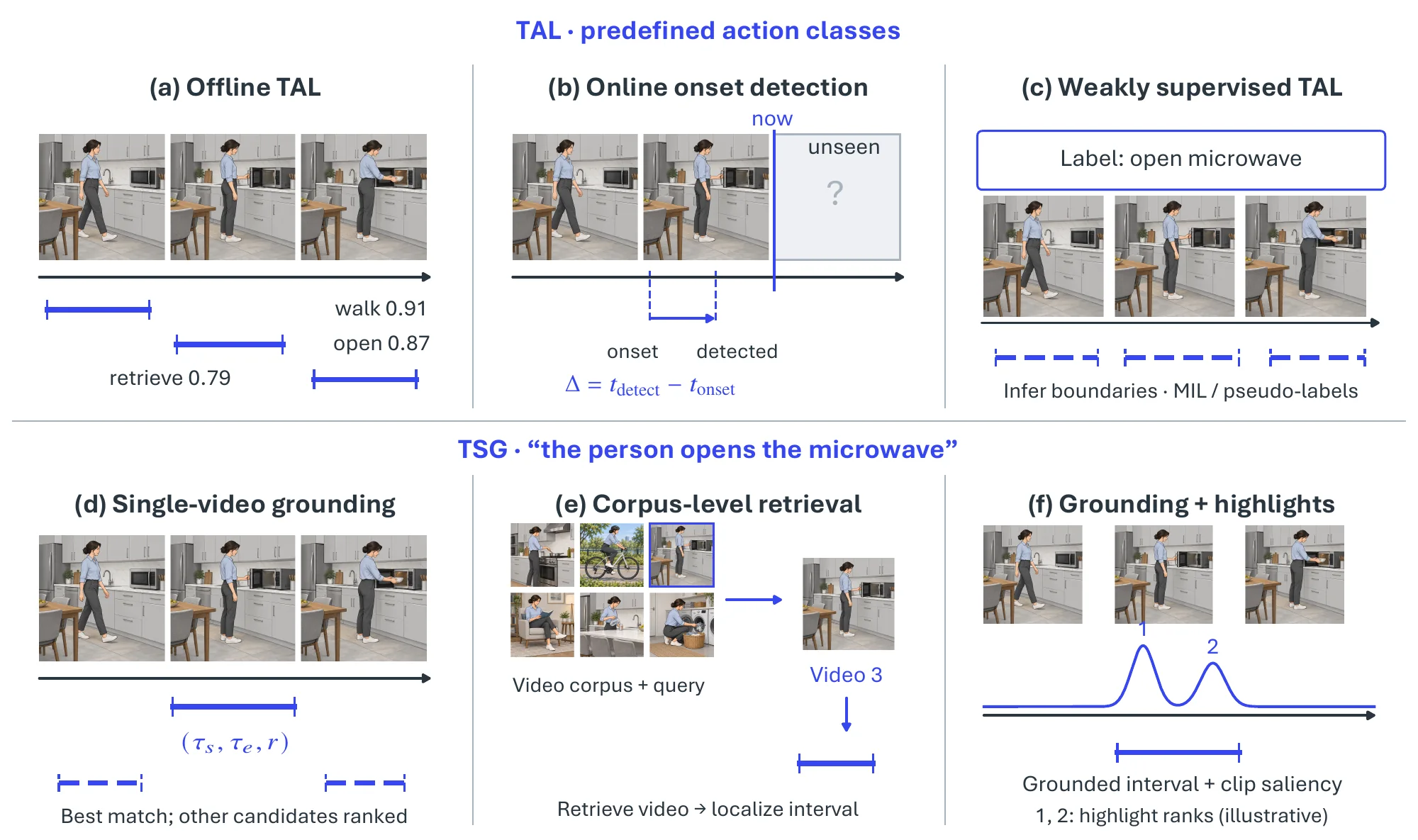
Temporal localization answers when something happens in a long, untrimmed video. The condition can be a category from a closed set, which gives temporal action localization (TAL) as treated in Section 6.3.4, or a free-form sentence, which gives temporal sentence grounding (TSG): return the segment that best matches “the person opens the microwave”. This subsection sets the two side by side, with the weight on the text-conditioned problem, which turns localization from exhaustive detection into retrieval and is what video search and interactive navigation [1033, 1034, 1035] rely on.
6.4.3.1Task Definition#
Temporal Action Localization (TAL) takes an untrimmed video , where may be a visual, audio, or multimodal feature, and detects all instances of predefined action classes, returning with : start and end times, a class label , and a confidence (the tuples of Section 6.3.4).
Temporal Sentence Grounding (TSG), also called natural language video localization or video moment retrieval, pairs with a sentence and returns a ranked list of moments , , with boundaries and a relevance score ; usually one segment is the answer. TAL is thus an exhaustive detection task over a closed label set, TSG a targeted retrieval task guided by open-ended language.
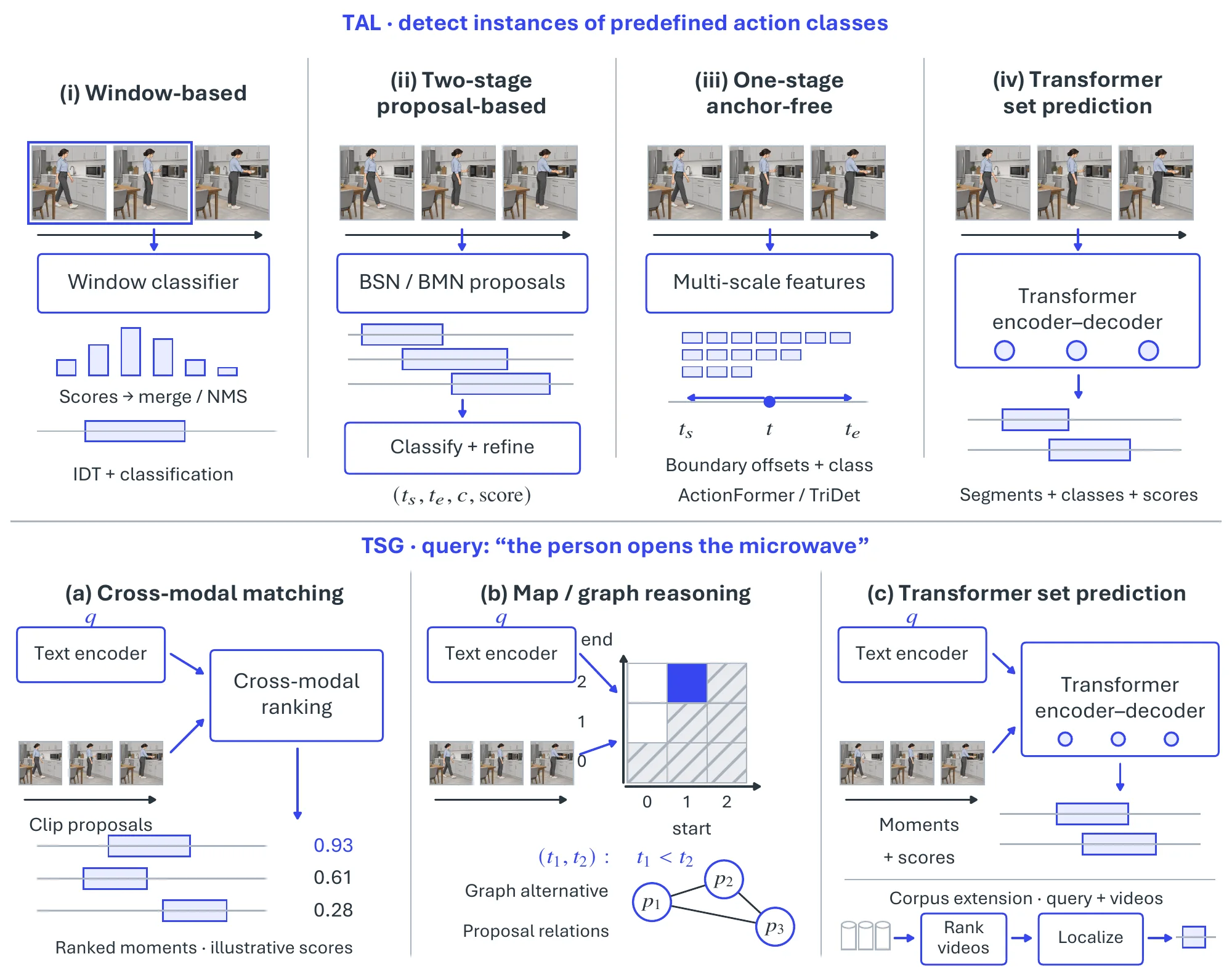
Both are studied under several settings, which Figure 6.25 lays side by side. Offline methods see the whole video; online methods infer causally over the streamed prefix and are judged on low-latency detection of action starts [1036, 1037]. Supervision ranges from frame-accurate boundaries to video-level labels only (weakly supervised TAL via multiple-instance learning, Section 6.3.4; weakly supervised TSG by aligning the two modalities during training [1038]), with self-supervised video pretraining [1039, 1040] and open-vocabulary or zero-shot variants [1041] reducing the labeled data needed. TSG additionally varies in scope, from a single video [1034, 1033] to corpus-level retrieval that first finds the video and then the moment (VCMR) [1042], and in output, with QVHighlights [1043] asking for a saliency ranking of highlight clips alongside the grounded moment.
6.4.3.2Methodology#
Figure 6.24 traces both tasks along the same path from hand-designed pipelines to end-to-end Transformers.
The TAL row is the detection lineage of Section 6.3.4: sliding windows over hand-crafted features such as improved dense trajectories [1044], then two-stage proposal-plus-classification systems (R-C3D [1045], SSN [883], TAL-Net [1046]) with dedicated boundary-sensitive proposal generators (BSN [884], BMN [1047], G-TAD [1048]), then anchor-free dense detectors and query-based set prediction. Three developments go beyond that treatment. Dense single-stage detectors were scaled by ActionFormer [1049], a multi-scale Transformer encoder over the feature pyramid, and TriDet [1050], which replaces self-attention with a convolutional scalable-granularity-perception module and a trident boundary head; both still regress boundaries at every position and rely on non-maximum suppression. DETR-style set prediction removes anchors and suppression: RTD-Net [1051] applies a relaxed Transformer decoder to proposal generation and TadTR [1052] decodes the full action set end to end [1053, 1054]. And masked video pretraining [1039, 1040] now supplies the backbones that these heads are fine-tuned on.
TSG began with cross-modal matching. CTRL [1034] embeds the sentence and candidate clips in a shared space and ranks clips, with boundary regression on top; MCN [1033] does the same for DiDeMo with global video context. Later models reason over the candidates jointly: MAN [1055] refines moments iteratively through a graph over proposals, 2D-TAN [1056] scores every (start, end) pair on a two-dimensional temporal-adjacency map so that neighboring candidates inform each other, and VSLNet [1057] drops proposals altogether and predicts the start and end positions as span extraction, in analogy to reading comprehension. Moment-DETR [1058] brought set prediction to grounding, decoding moments and saliency scores directly from an encoder–decoder, while TVR [1042] extended grounding to corpus scale with a coarse-to-fine search over subtitles and frames.
6.4.3.3Datasets and Metrics#
Table 6.29 lists the benchmarks; the TAL rows are those of Section 6.3.4, retained for comparison. The TSG benchmarks move from a closed domain (TACoS [1059], cooking) to open-domain sentences over indoor activity (Charades-STA [1034]), Flickr videos with multiple references per query (DiDeMo [1033]), and dense paragraph-level captions (ActivityNet Captions [1035]); YouCook2 [1060] adds procedural structure, TVR [1042] multimodal (subtitle) context and corpus-level retrieval, and QVHighlights [1043] saliency labels for joint highlight detection.
| Task | Dataset | Year | Scale / Classes | Temporal annotations |
| TAL | THUMOS14 [905] | 2014 | 200 train + 213 test videos / 20 cls | Frame-accurate, untrimmed |
| TAL | ActivityNet v1.3 [906] | 2016 | 20k videos / 200 cls | Untrimmed, diverse |
| TAL | HACS Segments [907] | 2019 | 50k videos / 200 cls; 139k segments | Clip+segment, dense |
| TAL | EPIC-KITCHENS-100 [1061] | 2020 | 700 egocentric videos / verb-noun labels | Egocentric, narration-aligned |
| TAL | MultiTHUMOS [909] | 2015 | 400 videos / 65 cls; 38.7k ann. | Dense, multi-label |
| TAL | FineAction [908] | 2022 | 17k videos / 106 cls; 103k instances | Fine-grained, precise |
| TSG | TACoS [1059] | 2013 | 127 cooking videos; 18.8k query-segment pairs | Cooking, aligned |
| TSG | Charades-STA [1034] | 2017 | 6.6k videos; 16,128 pairs | Charades-based pairs |
| TSG | DiDeMo [1033] | 2017 | 10k Flickr videos; 40k queries | Multi-reference, ranking |
| TSG | ActivityNet Captions [1035] | 2017 | 20k videos; 100k sentences | Dense captions |
| TSG | YouCook2 [1060] | 2018 | 2k untrimmed cooking videos / 89 recipes | Cooking procedures |
| TSG | TVR [1042] | 2020 | 21.8k clips (60–90 s) from 6 TV shows; 109k queries | Subtitles, multimodal |
| TSG | QVHighlights [1043] | 2021 | 10k YouTube videos; query+saliency | Query-saliency, highlights |
Temporal IoU between a predicted and a ground-truth segment is the primitive for both tasks, and TAL is scored by mAP at fixed tIoU thresholds (per-threshold on THUMOS14, averaged over on ActivityNet) and by AR@AN for proposal quality [1062], as defined in Section 6.3.4. TSG uses retrieval metrics instead. For queries , ranked predictions , and reference segments ,
| (6.43) |
is the fraction of queries for which some top- prediction overlaps a reference by at least (commonly , ), and scores the top prediction alone; QVHighlights adds mAP over tIoU thresholds [1043]. Recall at a threshold binarizes overlap and ignores the quality of the ranking, which motivated ranking-sensitive alternatives such as AxIoU [1063], and annotator disagreement about where a described moment begins and ends puts a ceiling on how precisely any of these can be measured.
Table 6.30 gives R@1 results for the TSG methods above; TAL numbers are in the table of Section 6.3.4. Relational reasoning over candidates (2D-TAN) and span prediction (VSLNet) roughly doubled CTRL’s R@1 at tIoU 0.5 on Charades-STA and raised it by half again at 0.7, and Moment-DETR adds a further step on Charades-STA without proposals or suppression; its QVHighlights numbers are the reference point for joint grounding and highlight detection.
| Method | Design | Charades-STA | ActivityNet Captions | QVHighlights |
| R@1 0.5 / 0.7 | R@1 0.5 / 0.7 | R@1 0.5 / 0.7 (mAP) | ||
| CTRL [1034] | Clip–sentence matching | 23.6 / 8.9 | 29.0 / 10.3 | – |
| MAN [1055] | Iterative graph adjustment | 46.5 / 22.7 | – | – |
| 2D-TAN [1056] | 2D temporal-adjacency map | 39.7 / 23.3 | 44.5 / 26.5 | – |
| VSLNet [1057] | Span prediction | 54.2 / 35.2 | 43.2 / 26.2 | – |
| Moment-DETR [1058] | Set prediction | 53.6 / 31.4 | – | 52.9 / 33.0 (30.7) |
6.4.3.4Challenges#
Boundaries are soft. Actions span sub-second gestures to multi-minute activities, which no single temporal resolution serves, and annotators disagree about where an instance starts and ends; a sentence adds its own ambiguity about which part of an activity it describes. The tIoU-thresholded metrics treat these fuzzy boundaries as exact, so part of the measured error is irreducible [1063], and probabilistic boundary modeling with calibrated confidences is the natural response.
The two tasks are converging. A closed label set limits TAL, while TSG is bounded by the vocabulary of its query sets; text prompts in place of class labels [1041] and set prediction for moments [1058] point to a single architecture that grounds both categories and sentences. Doing this over minutes of video, across camera viewpoints (egocentric footage in particular), with audio, narration, or noisy subtitles as further evidence [1042, 1043], and causally for streaming use [1036] is where the current systems fall short: memory-efficient long-context encoders and corpus-scale coarse-to-fine retrieval are the two ingredients most actively developed.