Recognition says what is present; it does not say where. Spatial localization and position estimation supply the missing geometry, situating recognized entities in a metric frame and recovering how they are oriented within it. The section climbs a ladder of geometric abstraction: from the per-pixel quantities of depth and surface normals, through metric attributes such as height and distance, to full SE(3) pose, first of the moving camera and then of rigid objects in the scene. Throughout, the concern is the static geometry of a single instant; how these quantities evolve is deferred to spatio-temporal perception.
6.2.1Depth Estimation#
Depth estimation predicts, for every pixel, the distance from the camera to the surface it observes, turning a 2D image into the 3D structure that reconstruction, navigation, and manipulation build on. Figure 6.6 summarizes the input configurations and the method families surveyed below.
6.2.1.1Task Definition#
Given an image and optional auxiliary observations (a second view, a multi-view set, a sparse sensor measurement, or neighboring video frames), a depth estimator predicts a depth map
| (6.13) |
where is the distance along the optical axis from the camera center to the surface seen at pixel . The task splits along three axes.
Sensing. Active methods emit light (structured light, time-of-flight, LiDAR) and measure its return, providing reliable metric depth even on textureless surfaces but tying accuracy to the sensor and degrading under strong ambient light or at long range. Passive methods infer depth from ordinary images alone; they need no special hardware and have become the dominant research line, at the cost of sensitivity to texture and illumination.
Scale. Metric depth gives distances in physical units, which 3D reconstruction and navigation require. Relative depth recovers only pixel ordering, or depth up to an affine transform; it cannot support metric measurement but is easier to supervise and generalizes better because heterogeneous datasets can be mixed without a consistent scale.
Density and Input Configuration. Classical pipelines produced sparse depth at feature points or semi-dense depth along high-gradient edges; dense per-pixel prediction is now the norm. The input configuration fixes how much geometry is available: active sensing measures depth directly; stereo recovers it from the disparity between two calibrated views; multi-view estimation enforces consistency across many views, which improves robustness to occlusion and matching ambiguity at the price of computation and known camera poses; monocular estimation has no geometric constraint at all and relies on learned statistical, structural, and semantic cues, which is why it is ill-posed in scale yet the most widely applicable setting.
6.2.1.2Methodology#
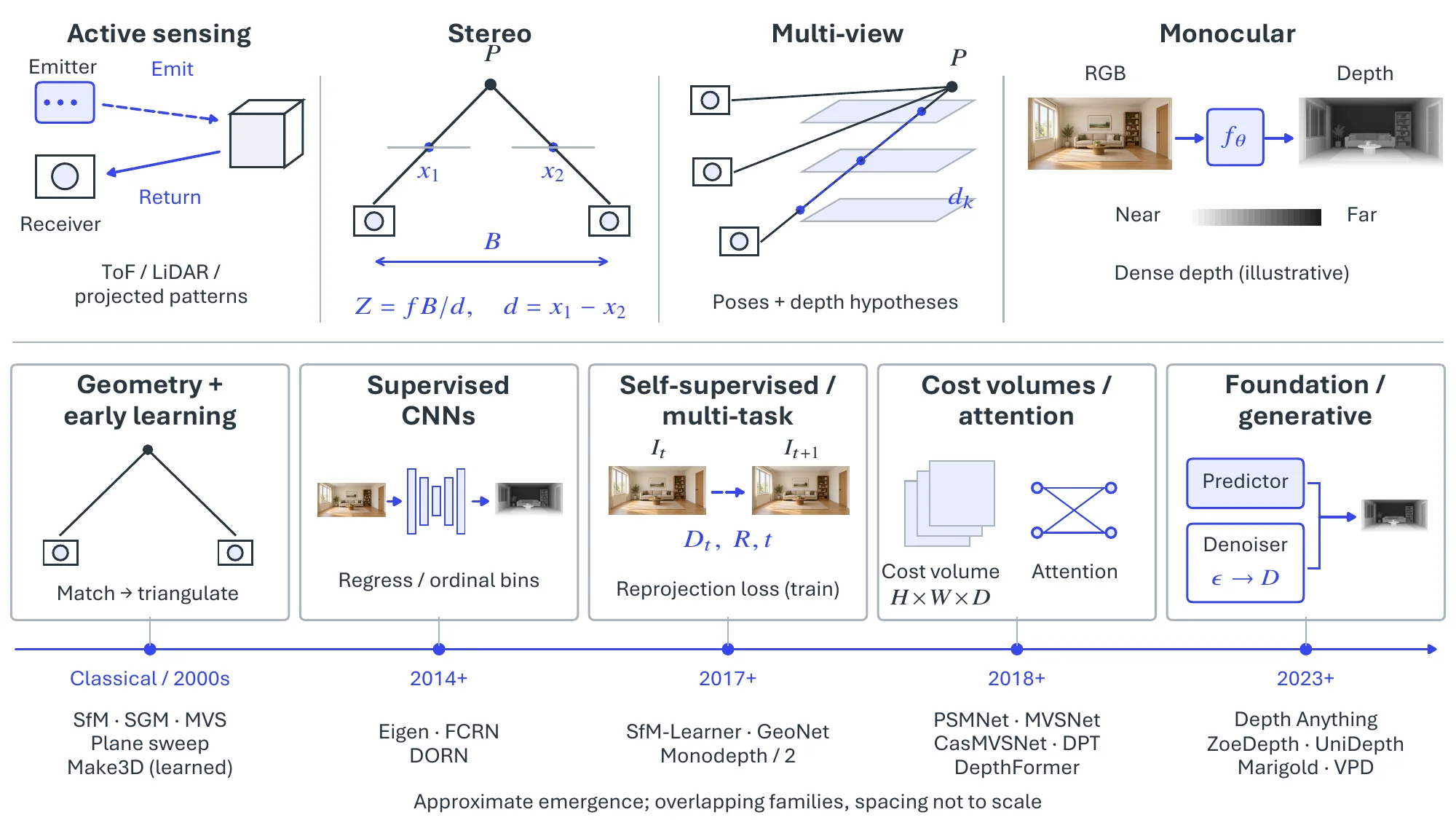
Geometric Methods. Classical depth estimation solves geometry explicitly. In binocular stereo, two rectified cameras with focal length and baseline observe a point whose projections differ by the disparity ; similar triangles give
| (6.14) |
so depth follows once correspondences are found. Stereo matching is therefore a correspondence problem, usually posed as an energy that balances data fidelity against smoothness; Semi-Global Matching approximates the global optimum by aggregating costs along several 1D paths and remains a standard dense baseline. Structure from Motion (SfM) extends triangulation to many uncalibrated views, recovering camera poses and a sparse point cloud up to global scale, and supplies the poses that Multi-View Stereo (MVS) densifies. MVS typically proceeds by plane sweep: for a reference pixel and a hypothesized depth , back-project with the intrinsics , transform into a source view with the relative pose , reproject, and keep the depth whose reprojections are most photometrically consistent across source views,
| (6.15) |
Plane sweep is thus triangulation turned into a search over depth planes, and it is the template that MVSNet [116] and CasMVSNet [613] later made differentiable as learned cost volumes.
Two single-image cues complete the classical picture. Depth from defocus exploits the thin-lens relation : a point off the focal plane blurs into a circle of confusion whose diameter grows with its distance from that plane, so measured blur can be inverted for depth. Shape from shading inverts a reflectance model, typically Lambertian, to recover surface orientation from intensity and integrates it into depth; it is treated under surface normals in §6.2.2. Both are ill-posed under unknown illumination, reflectance, or optics and survive today mainly as auxiliary cues.
Active Depth Sensing. Active sensors measure depth rather than infer it. Time-of-flight systems time the round trip of emitted light: LiDAR scans the scene with laser beams and returns a sparse but long-range point cloud, whereas ToF cameras flood the scene and recover a dense depth map at every pixel, best suited to short-range indoor use. Structured light projects a coded pattern (the Kinect v1 used a pseudo-random infrared speckle) and triangulates from its deformation; active stereo projects texture onto the scene only to make ordinary stereo matching stable on featureless surfaces.
Early Learning-Based Methods. Data-driven depth began in the mid-2000s with monocular estimation. Saxena et al. [614] regressed depth from hand-crafted multi-scale features with a Markov random field enforcing spatial coherence, and Make3D [38] extended the model to the 3D position and orientation of scene patches while releasing a laser-scanned outdoor dataset that served as an early benchmark.
Supervised CNN Regression. Eigen et al. [55] first applied CNNs to monocular depth with a coarse-to-fine two-scale network, and their evaluation protocol became the standard; a follow-up [250] showed that the same architecture predicts depth, normals, and semantic labels with minor changes. Deep Convolutional Neural Fields [615] paired CNN unaries with a continuous CRF, FCRN [616] introduced a fully convolutional encoder–decoder with efficient upsampling of ResNet features, and DORN [617] recast depth as ordinal regression over a spacing-increasing discretization.
Learned Stereo and Multi-View Stereo. Learning entered the geometric pipelines first as a replacement for individual components: MC-CNN [618] computed stereo matching costs with a Siamese network in place of hand-crafted similarity. Mayer et al. [619] then showed that networks can regress disparity and scene flow end to end, and GC-Net [182] and PSMNet [620] embedded the cost volume and its regularization inside the network. The same move reached multi-view geometry with SurfaceNet [621] and MVSNet [116], which infer depth from several posed images, and R-MVSNet [622] and CasMVSNet [613] improved their memory footprint and resolution.
Self-Supervised and Multi-Task Learning. Ground-truth depth is costly, so a second line replaced it with geometric consistency. SfM-Net [623] and SfM-Learner [133] learn depth and camera motion jointly from unlabeled video by minimizing photometric reprojection error between adjacent frames; Monodepth [624] obtains the same signal from stereo pairs, and Monodepth2 [180] unifies both sources in one framework. GeoNet [625] adds optical flow to the joint estimate. Because all of these train a monocular network with stereo or multi-view supervision, the old separation between input configurations began to dissolve. Alongside, multi-task sharing (depth with semantic segmentation [626]), ImageNet-pretrained encoders with structural losses (DenseDepth [627, 124, 595]), local planar guidance (BTS [628]), and mixed-dataset training for zero-shot transfer (MiDaS [629]) each pushed accuracy and generalization.
Transformers and Foundation Models. Self-attention [141] gives every pixel access to global context, which helps precisely where local convolutions fail: textureless regions, occlusions, and large scenes. DPT [630] established the pattern of a Vision Transformer [142] encoder with a light dense decoder, and DepthFormer [631] combined global attention with local convolutional refinement. Scaling data and model size then produced depth foundation models that are trained once and transferred zero-shot: ZoeDepth [632] and Depth Anything [140] learn from large mixed corpora with flexible supervision and generalize across scenes and capture conditions without per-dataset adaptation.
Video and Generative Depth. Video adds temporal constraints. ManyDepth [633] aggregates neighboring frames into a cost volume at test time, whereas MonoViT [634] keeps the self-supervised video objective but strengthens single-frame reasoning with a Transformer. A separate line treats depth as conditional generation: VPD [635] showed that text-to-image diffusion backbones carry usable geometric features, Marigold [636] reframed monocular depth as conditional denoising and obtained globally coherent maps under hard conditions, and GeoWizard [637] extended the recipe to joint depth and normal prediction. The same diffusion-as-perception idea recurs for surface normals and object pose later in this section.
Event-Based Depth. Event cameras record asynchronous per-pixel brightness changes [638, 639], offering microsecond latency and high dynamic range where frame cameras fail. Early event-based depth relied on geometric constraints and temporal accumulation [640, 641, 642, 643]; learned event stereo [644, 645], event–image fusion [646, 647], and self-supervised or hardware-aware frameworks [648, 649, 650] followed. The line remains a niche complement for extreme dynamics; see the survey [651].
6.2.1.3Datasets and Metrics#
Table 6.9 groups the main datasets into Type I, which ship explicit depth maps for direct supervision, and Type II, which require depth to be derived from LiDAR, stereo, or SfM. Three waves are visible. Indoor RGB-D collections (NYU Depth v2 [504], TUM RGB-D [652], SUN RGB-D [447], later ScanNet [448] and Matterport3D [340]) and the LiDAR-based KITTI [653, 654] fixed the indoor and outdoor protocols that still anchor the field, with Make3D [38] as the laser-scanned precursor. Relative-depth supervision from internet photos (DIW [655], ReDWeb [656], MegaDepth [657]) and synthetic data (Scene Flow [619]) then relaxed the need for metric sensors, while ETH3D [658], iBims-1 [659], ApolloScape [660], and Cityscapes stereo pairs [501] served precision evaluation and self-supervised training. The current wave is driven by autonomous driving and rendering: multi-sensor fleets (nuScenes [445], Waymo Open [446], Argoverse 2 [661], KITTI-360 [662], DDAD [663]) supply millions of LiDAR-calibrated frames, photorealistic synthetic sets (Hypersim [664], Virtual KITTI 2 [195], UrbanSyn [665], TartanAir [666]) supply exact ground truth even for transparent surfaces and hard lighting, and DIODE [667], BlendedMVS [668], ARKitScenes [669], Mannequin [670], and WildRGB-D [671] cover high-precision scans, handheld LiDAR, and dynamic or cluttered capture.
| Name | Year | Scene | Type | Metric | Setup | Volume | Data Source |
| Type I: Datasets with Explicit Depth Maps (Direct Supervision) | |||||||
| Make3D [38] | 2009 | Outdoor | Real | Metric | Mono | 534 | Laser Scanner |
| NYU Depth v2 [504] | 2012 | Indoor | Real | Metric | Mono | 1.4K | Kinect (SL) |
| TUM RGB-D [652] | 2012 | Indoor | Real | Metric | Mono | 39 Seqs | Kinect (SL) |
| SUN RGB-D [447] | 2015 | Indoor | Real | Metric | Mono | 10K | RGB-D Cameras |
| DIW [655] | 2016 | Varied | Real | Relative | Mono | 495K | Internet Photos |
| KITTI (Depth) [654] | 2017 | Outdoor | Real | Metric | Stereo | 93K | LiDAR (Velodyne) |
| ScanNet [448] | 2017 | Indoor | Real | Metric | Mono | 2.5M | Structure Sensor |
| Matterport3D [340] | 2017 | Indoor | Real | Metric | Mono | 194K | Matterport (RGB-D) |
| ETH3D [658] | 2017 | Both | Real | Metric | Multi-V | 13 Scans | Laser Scanner |
| ApolloScape [660] | 2018 | Outdoor | Real | Metric | Stereo | 140K | LiDAR + Stereo |
| iBims-1 [659] | 2018 | Indoor | Real | Metric | Mono | 100 | Camera + Laser |
| MegaDepth [657] | 2018 | Outdoor | Real | Relative | Mono | 130K | Internet + SfM |
| ReDWeb [656] | 2018 | Varied | Real | Relative | Mono | 3.6K | Internet + Stereo |
| DIODE [667] | 2019 | Both | Real | Metric | Mono | 26K | Camera + LiDAR |
| BlendedMVS [668] | 2020 | Both | Syn+Real | Metric | Multi-V | 17K | MVS Reconstruction |
| Hypersim [664] | 2020 | Indoor | Syn | Metric | Mono | 77K | Simulation |
| DDAD [663] | 2020 | Outdoor | Real | Metric | Multi-V | 76K | HD LiDAR |
| Virtual KITTI 2 [195] | 2020 | Outdoor | Syn | Metric | Stereo | 21K | Simulation (Unity) |
| TartanAir [666] | 2020 | Varied | Syn | Metric | Stereo | 1M | Simulation (UE4) |
| ARKitScenes [669] | 2021 | Indoor | Real | Metric | Mono | 5K Clips | iPad LiDAR |
| UrbanSyn [665] | 2023 | Outdoor | Syn | Metric | Mono | 7.5K | Simulation |
| WildRGB-D [671] | 2024 | Varied | Real | Metric | Mono | 20K | RGB-D Cameras |
| Type II: Datasets Requiring Depth to be Derived from Raw Geometry (LiDAR, Stereo or SfM) | |||||||
| KITTI (Raw) [653] | 2012 | Outdoor | Real | Metric | Stereo | 42K | LiDAR (Velodyne) |
| Cityscapes [501] | 2016 | Outdoor | Real | Metric | Stereo | 25K | Stereo Camera |
| Scene Flow [619] | 2016 | Varied | Syn | Metric | Stereo | 39K | Simulation (Blender) |
| NuScenes [445] | 2019 | Outdoor | Real | Metric | Multi-V | 1.4M | LiDAR |
| Waymo Open [446] | 2019 | Outdoor | Real | Metric | Multi-V | 200K | LiDAR |
| Mannequin [670] | 2019 | Varied | Real | Relative | Mono | 170K | Internet + SfM |
| KITTI-360 [662] | 2020 | Outdoor | Real | Metric | Stereo | 100K+ | LiDAR + Stereo |
| Argoverse 2 [661] | 2022 | Outdoor | Real | Metric | Multi-V | 6M | LiDAR |
Depth is evaluated with pixel-wise regression metrics. The root mean squared error and its logarithmic variant,
| (6.16) |
measure absolute deviation, the log form damping the dominance of far-range errors. Because an error of fixed size matters more at close range, relative errors normalize by the true depth,
| (6.17) |
and Abs Rel is the primary metric on most benchmarks. For monocular prediction, whose scale is ambiguous, the scale-invariant log error discounts a global scale shift,
| (6.18) |
Threshold accuracy reports the fraction of pixels within a multiplicative tolerance,
| (6.19) |
Ordinal metrics, which score only the pairwise depth ordering, are used where supervision is relative; they track perceived layout but say nothing about metric precision.
On KITTI, supervised regressors such as BTS [628] and DPT [630] reach Abs Rel around with near , while the self-supervised Monodepth2 [180] reaches Abs Rel near without any ground-truth depth. On NYU Depth v2, ZoeDepth [632] and Depth Anything [140] reach of and after fine-tuning, and UniDepth [672] matches them zero-shot, which makes transfer a credible alternative to per-benchmark training. Generative models such as Marigold [636] match or exceed regression on scale-invariant metrics while producing sharper boundaries, so recent gains come more from representation and data scale than from architectural depth. Boundary sharpness, temporal stability, and latency are still not evaluated in a standard way.
6.2.1.4Challenges#
Monocular depth is ill-posed: distinct 3D scenes project to the same image, so a single view fixes depth only up to scale and predictions drift across scenes. Scene content adds its own failures. Moving objects break the static-world assumption behind self-supervised and multi-view methods, and in video the result is flicker between frames and scale drift over time. Transparent and reflective materials and textureless regions give weak or misleading appearance cues; thin structures and sharp boundaries lose detail; low light, adverse weather, and underwater imagery degrade models trained on clean data. These scene effects compound into a domain gap: models are tied to the geometry and depth distribution of their training data, the indoor–outdoor divide is especially wide, real depth labels are scarce and noisy, and synthetic data still transfers imperfectly.
Current work attacks these problems from several sides. Depth foundation models [140, 672, 632] supply strong zero-shot priors, and Video Depth Anything [295] adds temporal modules to one of them for consistent video depth, while video depth diffusion (DepthCrafter [294], ChronoDepth [673], RollingDepth [674]) pursues the same goal generatively. Coupling depth with 3D scene representations (DepthSplat [675]) improves spatial consistency, language cues help anchor metric scale [676], and lightweight architectures such as MonoLENS [677] and LMDepth [678] target the real-time budgets of driving, robotics, and AR/VR.
6.2.2Surface Normal Estimation#
Surface normal estimation predicts the local orientation of visible surfaces from images or videos. Where depth answers “how far is this point from the camera?”, a normal answers “which way does the surface face?”. That makes normals a compact, scale-invariant description of local 3D geometry: a normal field exposes planes, folds, object boundaries, and contact surfaces even when metric depth is ambiguous, which is why it serves reconstruction [288], relighting and intrinsic decomposition [679, 248], physical interaction modeling [680], and egocentric perception [681].
The learning problem looks simple: from an RGB image, RGB-D frame, multi-view set, or video, output one unit vector per valid pixel. The inverse problem underneath is badly constrained, since the same intensity can be explained by different combinations of shape, reflectance, and illumination, and camera intrinsics change how image gradients map to 3D orientation. Progress has therefore come from three directions at once: more and better supervision, stronger geometric inductive biases, and visual priors inherited from large dense-prediction and diffusion models; since 2024 the last of these has turned normal estimation into one output head of broader geometric foundation models.
6.2.2.1Task Definition#
Let be an image, optional auxiliary observations (neighboring frames, stereo or multi-view images, depth, intrinsics, or poses), and the set of valid pixels. The goal is to estimate
| (6.20) |
where each is a unit vector in the camera frame or in a gravity- or world-aligned frame. Supervision comes from depth sensors, fitted meshes, rendered assets, multi-view reconstruction, or indirectly from photometric and intrinsic-image losses, and camera metadata matters because a pixel’s viewing ray depends on focal length and field of view. Monocular prediction from one RGB image is the canonical benchmark setting; RGB-D variants use measured or predicted depth as input or supervision through the differential relation between depth gradients and normals, multi-view and video variants enforce viewpoint or temporal consistency, object-centric variants target CAD-like objects, hands, faces, and bodies, and panoramic variants predict under equirectangular or fisheye geometry, where pinhole assumptions break.
6.2.2.2Methodology#
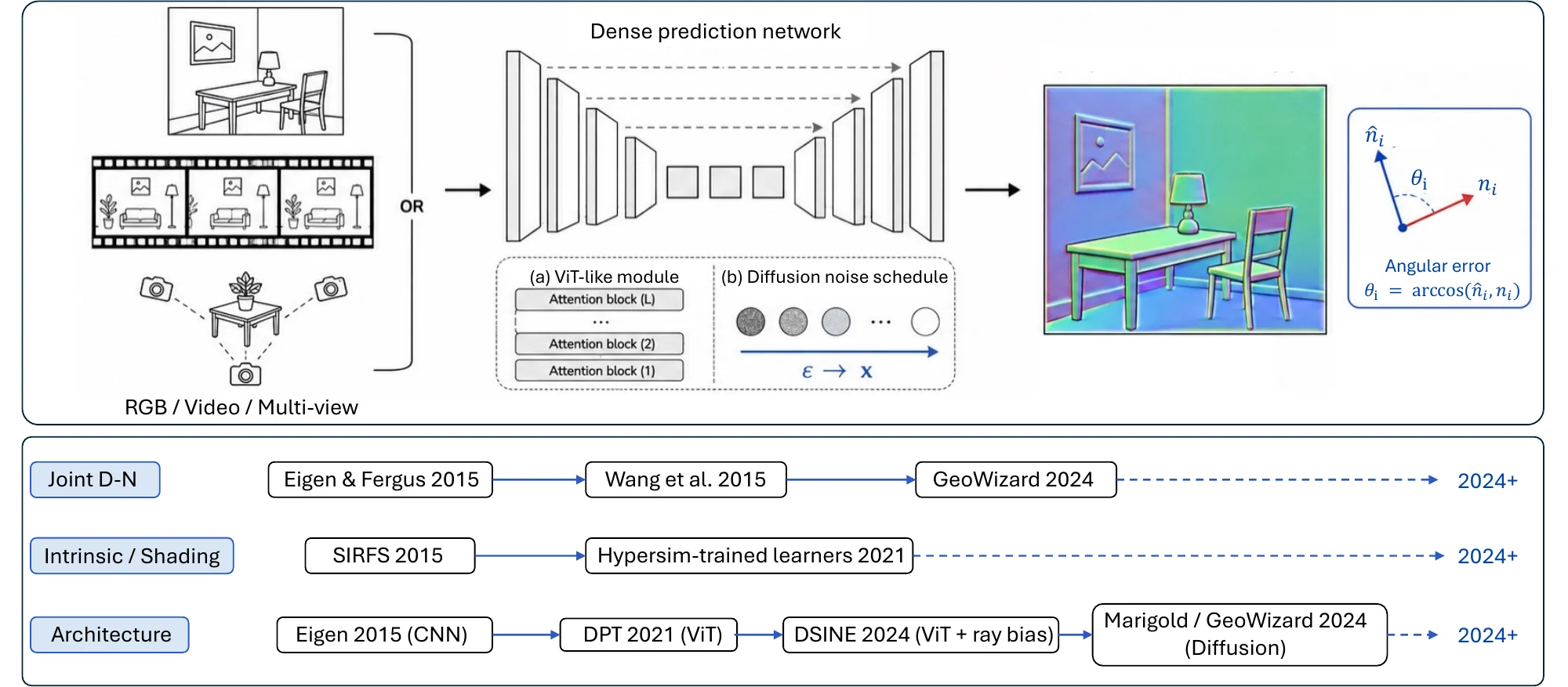
Surface normal estimation has moved from physics-based inverse rendering to supervised dense prediction and, most recently, to foundation-model and diffusion-based geometry estimation. Figure 6.7 summarizes the method families; the last two below are grouped as one family in the figure.
Photometric and intrinsic-decomposition methods. The classical origin is shape from shading and photometric stereo. Photometric stereo recovers orientation from several images taken under different lighting; Woodham’s formulation [249] shows that normals follow once illumination and reflectance are sufficiently constrained. Single-image shape from shading is harder because a change in intensity may signal a change in orientation, albedo, illumination, or material; SIRFS [248] is the canonical optimization-era method, jointly recovering shape, illumination, and reflectance under natural-image and geometric priors. These methods identify the physical ambiguities that every later learned model inherits, and physically based rendering datasets such as Hypersim [664], where shading, materials, depth, and normals are jointly available, keep their logic in play.
Supervised CNN and multi-task dense prediction. Eigen and Fergus [250] trained one multi-scale convolutional network to predict depth, normals, and semantic labels, establishing that normals can be regressed directly from RGB and that geometric tasks benefit from shared representations. Later CNN systems improved encoder capacity, decoder resolution, and boundary preservation, usually with normals as one branch of a multi-task perception model, and Taskonomy [682] and Omnidata [683] systematized the paradigm by training dense predictors across many 3D scans and tasks. A CNN normal estimator runs in one forward pass and drops into real-time reconstruction, AR, or robotics pipelines; its local features, however, blur thin structures and lack the global context needed for consistent orientation across large planes.
Transformer and camera-aware discriminative predictors. Vision Transformers let every output pixel attend to the whole image. DPT [630] showed that Transformer features support strong dense prediction across depth and semantics, and the same global context helps normals: co-planar walls, floors, and object faces may be far apart in the image yet geometrically coupled. Pure attention discards one geometric fact, that pixels correspond to camera rays; DSINE [684] injects ray-direction information and shows that camera geometry remains valuable even for large learned backbones.
Diffusion and foundation-model priors. A more recent line casts normal estimation as conditional generation or as one head of a general geometric foundation model. VPD [635] showed that text-to-image diffusion models carry useful features for dense perception, and GeoWizard [637] extended the Marigold recipe of §6.2.1 to joint depth and normal prediction under a shared generative prior. Metric3Dv2 [685] took the discriminative route, training a camera-aware monocular model for metric depth and normals across heterogeneous datasets. StableNormal [686] addressed a practical weakness of diffusion-based normals: stochastic denoising yields high-quality but high-variance maps, so reducing variance matters as much as improving the mean. The generative formulation samples uncertain or textureless regions from a learned distribution instead of forcing a single local regression, at the cost of iterative-denoising latency, which motivates distillation and single-step variants.
Temporal, multi-view, and reconstruction-coupled methods. Normals matter most when predictions must persist across time or support 3D reconstruction. Video normal estimation enforces temporal consistency by warping predictions with optical flow or camera poses and penalizing flicker; NormalCrafter [687] targets temporally consistent sequences for downstream video reconstruction and editing rather than per-frame accuracy alone. Multi-view settings derive normals from reconstructed meshes or regularize them through cross-view photometric consistency, and neural surface reconstruction such as NeuS [288] consumes normal-like differential geometry implicitly through signed-distance gradients, so normal estimation and reconstruction now supervise each other.
Material- and domain-specific normal estimation. A smaller branch revisits what generic models still get wrong. Transparent, reflective, and laboratory objects violate Lambertian assumptions because their gradients come from refraction, reflection, or the background rather than the surface; TransNormal [688] targets transparent objects with a dedicated benchmark and model, making explicit that open-world normal prediction cannot be solved by indoor RGB-D supervision alone.
| Dataset | Year | Domain | Source | Normal supervision / use |
| NYU Depth v2 [504] | 2012 | Indoor | RGB-D | Normals derived from Kinect depth; canonical indoor monocular normal benchmark. |
| SUN RGB-D [447] | 2015 | Indoor | RGB-D | Depth-derived normals across diverse indoor scenes and sensors. |
| ScanNet [448] | 2017 | Indoor | RGB-D video + mesh | Mesh- or depth-derived normals with camera trajectories; useful for video and reconstruction-linked supervision. |
| Matterport3D [340] | 2017 | Indoor panorama | RGB-D scans + mesh | High-resolution reconstructed geometry; supports room-scale and panoramic normal evaluation. |
| Taskonomy [682] | 2018 | Indoor | 3D scans | Large multi-task supervision including surface normals, depth, reshading, and semantics. |
| Replica [339] | 2019 | Indoor synthetic / scanned | Rendered geometry | Clean normals from high-quality reconstructed scenes; useful for controlled evaluation. |
| DIODE [667] | 2019 | Indoor / outdoor | LiDAR depth | Depth-derived normals; stresses cross-domain generalization beyond NYU-style indoor scenes. |
| Hypersim [664] | 2021 | Indoor synthetic | PBR rendering | Ground-truth depth, normals, materials, and lighting for geometry + intrinsic learning. |
| Omnidata [683] | 2021 | Indoor multi-source | 3D scans | Large-scale mid-level vision training data with normals and many related tasks. |
6.2.2.3Datasets and Metrics#
Table 6.10 shows that normal supervision is usually inherited from another representation rather than annotated directly. RGB-D datasets (NYU Depth v2 [504], SUN RGB-D [447], ScanNet [448]) supply measured depth from which local planes or mesh normals are computed, which fixes the indoor evaluation regime but also means the labels are only as good as the depth sensor and are dominated by man-made indoor structure. Scanned and synthetic collections address coverage and label quality from opposite sides: Matterport3D [340], Taskonomy [682], and Omnidata [683] scale supervision across many environments and tasks, whereas Replica [339] and Hypersim [664] give clean rendered normals with physically meaningful lighting at the price of a synthetic-to-real gap. DIODE [667] pushes toward indoor–outdoor generalization, yet outdoor normals remain far less standardized than outdoor depth because sparse LiDAR is a poor match for dense orientation supervision; intrinsic-image sets such as IIW [689] and MPI Sintel Intrinsics [690] constrain shading and reflectance for inverse-rendering formulations without being normal benchmarks themselves. The most visible gap is temporal: although ScanNet and other RGB-D videos contain sequences, there is no widely adopted video normal benchmark, so temporal stability is reported qualitatively or through method-specific warping losses, even though flicker often hurts reconstruction and AR consumers more than a small rise in mean angular error.
Evaluation is angular because normals are unit vectors. With the predicted and ground-truth normals at valid pixel and the number of valid pixels, the per-pixel error in degrees is
| (6.21) |
summarized by its mean (sensitive to boundary noise and invalid-depth artifacts), its median (robust to a few severe failures), occasionally its RMSE, and by threshold accuracies
| (6.22) |
which expose changes in the fraction of practically usable pixels that a small shift in mean error can hide. Training objectives usually minimize the cosine loss , monotonic in angle for unit vectors, but benchmarks report angles for interpretability. Beyond per-pixel angle, joint depth–normal models are checked for agreement between predicted normals and normals differentiated from depth, reconstruction-oriented work asks whether normal discontinuities align with object boundaries and whether large planes stay coherent, and video methods report temporal consistency by warping predictions between adjacent frames with flow or pose,
| (6.23) |
after rotating camera-frame normals into a common frame. Protocol details move rankings: depth-derived normals are unstable at discontinuities, papers mask invalid pixels differently, and some evaluate in the camera frame while others rotate into a gravity-aligned frame, so the table below records which paper produced each number.
| Method | Family | Year | Mean | Median | |
| Eigen & Fergus [250] | Multi-scale CNN, multi-task | 2015 | 20.9 | 13.2 | 44.4 |
| Omnidata [683] | Large-scale mid-level supervision | 2021 | 23.1 | 12.9 | 45.8 |
| DSINE [684] | Ray-aware discriminative | 2024 | 16.4 | 8.4 | 59.6 |
| Metric3Dv2 (ViT-g, zero-shot) [685] | Geometric foundation model | 2024 | 13.3 | 7.0 | 66.4 |
| Marigold (normal variant)† [636] | Diffusion prior | 2024 | 20.9 | 11.1 | 50.5 |
| GeoWizard† [637] | Joint depth + normal diffusion | 2024 | 20.4 | 11.9 | 47.0 |
| StableNormal† [686] | Low-variance diffusion | 2024 | 19.7 | 10.5 | 53.0 |
Table 6.11 makes two things visible. Within one protocol, camera-aware discriminative models lead: DSINE roughly halves the median error of the 2015 baseline, and Metric3Dv2 reaches mean error zero-shot, so projective inductive bias and large camera-diverse pretraining still pay off even with strong backbones. Diffusion-based estimators trail these numbers on NYU Depth v2 under the StableNormal protocol, but they trade accuracy on clean indoor scenes for coherence in textureless or ambiguous regions and for a usable uncertainty, which the single-frame benchmark does not reward; the post-GeoWizard line has accordingly shifted the target from single-frame accuracy toward stable, usable geometry, StableNormal controlling diffusion variance and NormalCrafter [687] enforcing temporal coherence.
6.2.2.4Challenges#
An RGB image alone does not determine shape, lighting, and reflectance: a dark pixel may be a tilted surface, a dark material, a cast shadow, or a specular highlight, and learned models resolve the ambiguity with priors rather than removing it, which is why estimators look confident on common indoor layouts and fail systematically on rare materials, unusual lighting, and out-of-distribution scenes. The persistent failure modes follow from this. Reflective and transparent surfaces produce gradients caused by the environment rather than the surface. Textureless and weakly lit regions give little evidence, and networks hallucinate planar sheets. Thin structures and depth discontinuities mix receptive fields and inherit depth-derived label noise, blurring normals around chair legs, plants, railings, and silhouettes. Wide-field and panoramic cameras break models trained under narrow pinhole assumptions, which is what makes ray-aware designs such as DSINE [684] necessary. Dynamic and deformable objects flicker because most supervision comes from static scans or rigid synthetic scenes.
Dataset bias compounds the problem: canonical benchmarks are indoor and sensor-derived, so outdoor surfaces, hands, faces, deformable and transparent objects, and egocentric manipulation stay underrepresented, and no accepted benchmark jointly measures cross-domain generalization, temporal stability, and downstream reconstruction quality. TransNormal [688] is a corrective for one slice of the non-Lambertian regime (glass, liquid, mirror, metal, wet roads), which remains far from solved. The directions now taking shape answer these gaps directly: geometric foundation models that merge depth, normals, segmentation, material, and calibration into one dense-prediction backbone, following Omnidata [683] through Metric3Dv2 [685] and GeoWizard [637]; diffusion distillation and variance control that keep the coherence and uncertainty of generative models while recovering real-time, deterministic inference [686]; temporally consistent, reconstruction-coupled normals [687]; and physically grounded models for non-Lambertian materials, where data scale is no substitute for modeling refraction and reflection.
6.2.3Height and Distance Estimation#
Height and distance estimation recovers absolute, real-world lengths: the dimensions of an object (the height of a person), the separation between scene entities (the gap between two vehicles), or the displacement of a moving object over time, from which speed follows. Whereas depth estimation (§6.2.1) recovers a dense per-pixel distance from the sensor to every visible surface, height and distance estimation targets a few metric quantities defined between scene entities rather than relative to the sensor, and is therefore tied to specific object instances and to a downstream measurement requirement. Radar, ultrasonic, and radio ranging measure such distances directly and are mature; this subsection covers the vision-based problem.
6.2.3.1Task Definition#
The input is one or more images or a video together with a specification of what to measure: the height of an object, the distance between two objects, or the distance an object travels. The output is a length in physical units, or a displacement over a time interval, from which average speed is read off (speed estimation).
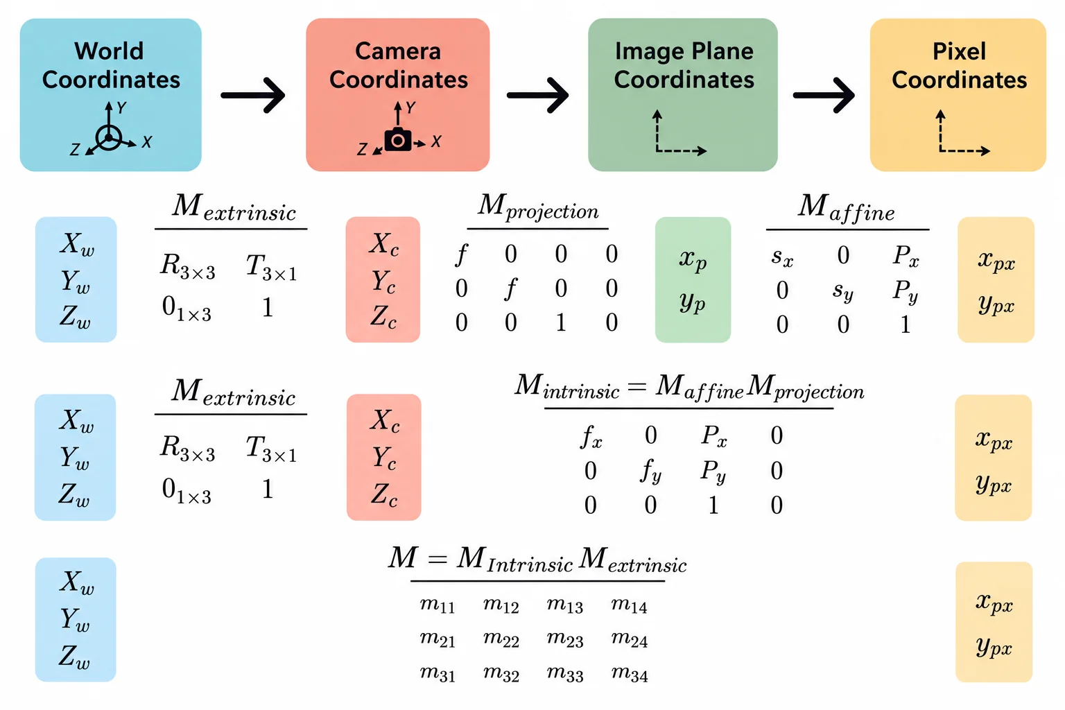
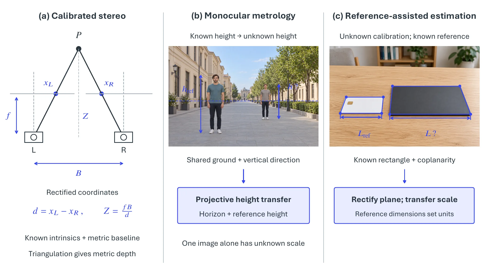
Every vision-based route to a metric length passes through the camera model, shown in Figure 6.8. Under the pinhole model a world point with homogeneous coordinates projects to the pixel
| (6.24) |
where the extrinsics move the point into the camera frame and the intrinsic matrix (focal length, principal point, pixel aspect) maps metric image-plane coordinates to pixels. Real lenses deviate from this model; Brown’s model [691] corrects the dominant radial term as
| (6.25) |
with a tangential term for sensor–lens misalignment, and camera calibration [692] recovers together with the distortion coefficients. Without calibration, every pixel-to-length conversion inherits an unknown scale.
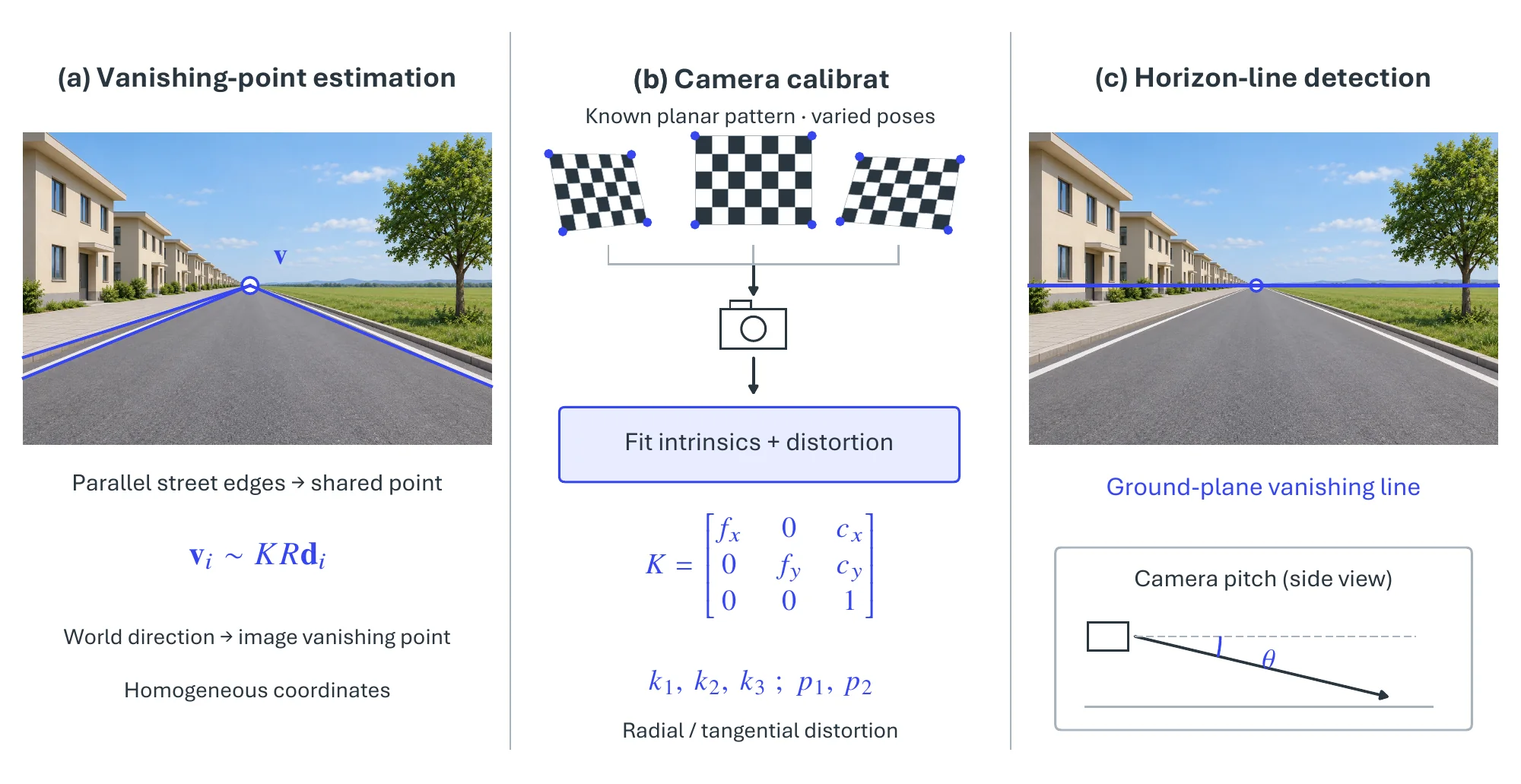
Beyond calibration, geometric pipelines rely on a small set of recurring intermediate quantities, illustrated in Figure 6.9: vanishing points, where parallel world lines converge and from which camera orientation follows; the horizon line, which fixes the camera’s tilt relative to the ground; and a ground-plane homography, which lets lengths on a dominant plane such as a road or floor be measured once a single reference length is known. Stereo pipelines add rectification, which aligns the two image planes so that correspondences lie on the same scanline, and disparity matching. Learning-based pipelines keep object detection (Section 6.1.1) as the front end and replace the explicit geometry with regression of depth, 3D center, and dimensions from region features, optionally conditioned on a dense depth map and refined over time when video is available.
6.2.3.2Methodology#
Vision-based height and distance estimation is organized along two axes: the sensor configuration (stereo versus monocular), which decides whether metric depth is available by triangulation, and the inference paradigm (geometry-based versus learning-based), which decides whether scene geometry is solved from projective constraints or inferred from data. Figure 6.10 lays out the resulting families; it draws the uncalibrated case as a third branch for readability, but it is best read as the weakly constrained regime of monocular or stereo inference in which some geometric information is missing and must be supplied by priors.
Stereo Vision. A calibrated stereo rig recovers metric depth directly from disparity, with focal length , baseline , and disparity . Classical pipelines run calibration, rectification, matching, disparity estimation, and triangulation [692, 693, 112]; their accuracy rests on calibration quality and on matching reliability in textureless, reflective, or occluded regions, and object distance is read off by aggregating depth over the detected region. Multi-view stereo adds views for consistency without changing the triangulation principle [694, 116]. Learned stereo replaces hand-crafted matching costs with learned features and cost volumes [182, 620, 695] and, in recent systems, folds distance estimation into stereo 3D object detection, predicting category, 2D extent, depth, and 3D box jointly [696, 697, 698]. Learning improves robustness, but the metric scale still comes from the calibrated baseline and intrinsics.
Monocular Vision. A single image does not fix absolute scale, so monocular methods recover it from explicit geometric constraints, learned priors, or external reference information [112, 699]. Classical monocular metrology uses projective geometry: vanishing points of parallel world lines give camera orientation [700, 112], and a homography between a dominant ground plane and the image enables metric measurement on that plane once one reference length is known [699, 701]. The approach is interpretable and accurate in controlled scenes but needs clean geometric cues, reliable calibration, and visible parallel lines or planar supports. Learning-based monocular methods detect objects in 2D and regress their depth, 3D center, and physical dimensions directly from image features [702, 703, 704, 705, 706, 707, 708, 449], implicitly learning the inverse relation between image extent and distance together with perspective, context, and occlusion cues, without an explicit vanishing-point or homography step.
Foundation-Model-Assisted Metric Estimation. A newer route uses pretrained metric or metric-aligned depth models as an intermediate representation. DPT, ZoeDepth, Metric3D, and Depth Anything predict dense depth from a single image with strong cross-domain generalization [630, 632, 709, 140]; pooling the predicted depth inside a detected region or instance mask then gives object distance, and combining masks, depth, and simple geometric constraints gives object height. This removes the need for explicit vanishing-point detection and manual scene calibration and offers a practical path to metric estimation on in-the-wild images. In the fully uncalibrated case, exact metric recovery from one image remains ill-posed [112]; practical systems inject scale through a known reference object, a known camera height, a ground-plane assumption, category-level size priors, or one of the pretrained metric-depth models above [699, 703, 632, 709].
6.2.3.3Datasets and Metrics#
Table 6.12 summarizes the benchmarks, which fall into three groups by sub-task. Object-size estimation is evaluated on the indoor RGB-D sets CAMERA25 and REAL275 [710], where category-level dimensions are scored jointly with pose on controlled tabletop scenes. Sensor-to-object distance is rarely benchmarked on its own; it is evaluated through the 3D-detection annotations (box centers, sizes, velocities) of the driving datasets KITTI [653], nuScenes [445], Waymo Open [446], and Argoverse 2 [661], which test metric localization at scale across multi-camera rigs and scenes, with BDD100K [711] as a monocular video source. Speed and displacement estimation is dominated by fixed-camera traffic video: AI City Challenge 2018 [712], BrnoCompSpeed [713], UTFPR [223], and QMUL [714], plus the UAV-mounted Beihang videos [715]; these are the only benchmarks that score a physically meaningful motion quantity rather than static geometry.
| Dataset | Task | Modality | View | Domain | Scale | Resolution |
| CAMERA25 [710] | Size | RGB-D image | Monocular | Mixed-reality indoor | 300K images | - |
| REAL275 [710] | Size | RGB-D image | Monocular | Indoor | 8,000 images | - |
| KITTI 3D [653] | Distance | RGB + LiDAR | Monocular | Vehicle | 15K frames | - |
| nuScenes [445] | Size / distance | RGB + LiDAR + radar | Multi-view | Vehicle | 1,000 scenes | - |
| Waymo Open Dataset [446] | Size / distance | RGB + LiDAR | Multi-view | Vehicle | 1,150 segments | - |
| Argoverse 2 Sensor [661] | Size / distance | RGB + LiDAR | Multi-view | Vehicle | 1,000 scenes | - |
| AI City Challenge 2018 [712] | Speed | Video | Binocular | Vehicle | 45 hours | 19201080, 800410 @30 Hz |
| BrnoCompSpeed [713] | Speed | Video | Monocular | Vehicle | 18 videos 1 hour | 19201080 @50 Hz |
| UTFPR [223] | Speed | Video | Monocular | Vehicle | 5 hours | 19201080 @30 Hz |
| QMUL [714] | Speed | Video | Monocular | Vehicle | 1 hour | 360288 @25 Hz |
| Beihang UAV Videos [715] | Speed | Image | Monocular | Vehicle | 70 images | 960540 |
| BDD100K [711] | Size / distance | Video | Monocular | Vehicle | 100K videos | 720p @30 Hz |
Each sub-task is scored with the same triplet: an absolute error in physical units, a relative error for cross-range comparison, and a threshold accuracy for downstream binary decisions. For object size, the metric is the mean absolute error in physical units (centimeters for human height, millimeters for category-level pose),
| (6.26) |
with the mean absolute percentage error alongside for cross-class comparison; when size is scored jointly with pose, the 3D IoU of predicted and ground-truth boxes is thresholded, the NOCS protocol [710] reporting at IoU and at cm translation. Inter-object distance reuses MAE, RMSE, and MAPE on distances and the depth-style ratio accuracy of §6.2.1 with ; because stereo error grows as , KITTI-style protocols [653] stratify by range (near m, mid – m, far m) so that far-field degradation is not averaged away. Speed estimation reports MAE, RMSE, and MAPE in km/h, but the dominant device is a percent-within-tolerance band: AI City Challenge 2018 [712] fixes km/h and combines it with detection recall into its S1 score, and BrnoCompSpeed [713] adds the median absolute error because single-frame outliers from motion blur or detection jitter distort the mean. Two protocol details change rankings: per-vehicle averaging (BrnoCompSpeed) weighs trajectories differently from per-frame averaging matched to track IDs (AI City), and monocular and uncalibrated methods are sensitive to the assumed focal length, principal point, and reference length, so their reported accuracy is only meaningful together with the calibration assumptions.
Performance is sub-task specific. Category-level size recovery on REAL275 [710] remains far from millimeter accuracy in cluttered scenes. On BrnoCompSpeed [713], calibration-aware pipelines reach low single-digit km/h errors on the original sessions but degrade when transferred to unseen camera placements, exposing the brittleness of fixed-camera homography assumptions, and on the AI City 2018 speed track [712] the leading entries pair strong detection-and-tracking front ends with multi-frame speed regression, so the S1 score reflects detection recall as much as raw speed accuracy. Across all three sub-tasks the bottleneck is calibration, of the camera and of the scene-plane reference, rather than the regression backbone.
6.2.3.4Challenges#
Calibration sensitivity is the dominant open problem: small errors in intrinsics or in the scene-plane reference propagate non-linearly into every recovered length, and methods that treat focal length and reference size as latent variables, or refine calibration online from multi-view consistency, generalize across camera setups where fixed-calibration pipelines fail. The second gap is coverage: benchmarks are confined to indoor tabletop size estimation and vehicle-traffic speed, leaving pedestrian speed in crowds, package dimensions in logistics, and indoor inter-object distance essentially unmeasured. Fusing visual estimates with LiDAR, radar, or inertial sensing would lift robustness in low light and under occlusion, but the vision-only setting treated here still lacks a benchmark that scores metric accuracy jointly with calibration uncertainty.
6.2.4Visual Odometry and Camera Pose Estimation#
Visual odometry (VO) and camera pose estimation recover the position and orientation of a camera from visual observations. They provide the coordinate scaffold that lets a system stitch individual images into a persistent spatial representation: depth, surface normals, scene flow, maps, and 3D reconstructions all become more useful once they can be expressed in a shared camera or world frame. VO usually means estimating incremental motion between consecutive frames, often as a trajectory in ; camera pose estimation is broader and may recover a query image’s absolute 6-DoF pose in a known scene, the relative pose between two views, or camera motion and scene geometry jointly from an unordered image collection. The field was built on geometric optimization and SLAM, and its center of gravity is now shifting toward learned correspondence, differentiable optimization, dense geometric priors, and feed-forward geometric foundation models that predict cameras and geometry together.
6.2.4.1Task Definition#
Let denote the pose of camera with respect to a world frame. Given images (monocular, stereo, RGB-D, multi-view, or video), optional intrinsics , optional inertial readings, and sometimes a prior map or database, the goal is to estimate relative transformations , an absolute pose for a query image, or a full trajectory together with sparse or dense scene geometry, and occasionally the intrinsics themselves when calibration is unknown. The variants differ in what is assumed known. Monocular VO is scale ambiguous without external priors; stereo and RGB-D VO recover metric scale from a known baseline or measured depth; visual-inertial odometry uses IMU measurements to stabilize scale and fast rotation; SLAM adds mapping and loop closure to online odometry; SfM recovers poses and structure from unordered collections; map-based relocalization assumes an existing scene representation and places a query in it; and map-free relocalization and feed-forward reconstruction skip explicit map construction by predicting relative pose or globally aligned point maps directly from images.
6.2.4.2Methodology#
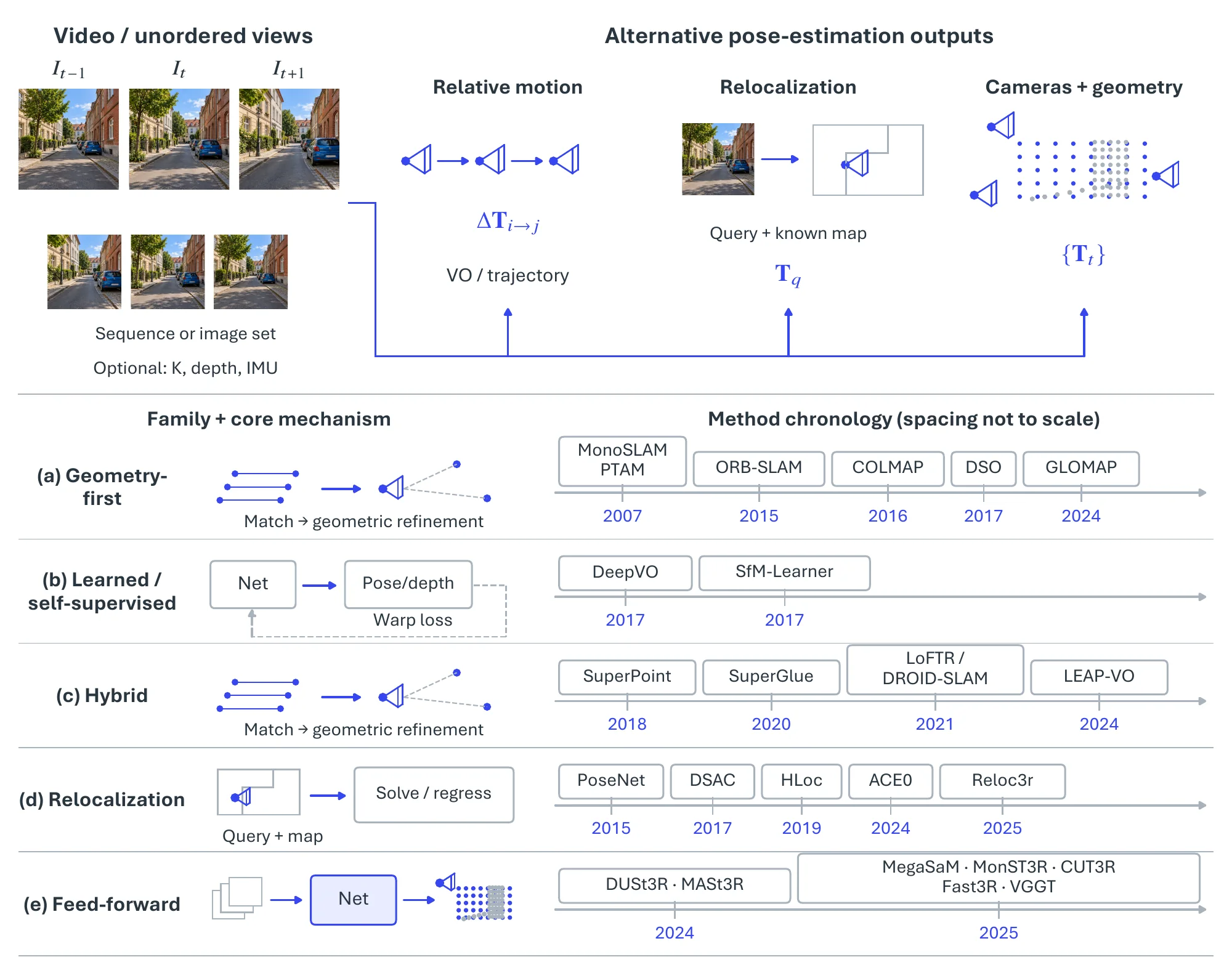
Figure 6.11 summarizes five method families, ordered from explicit geometry to learned geometric priors to feed-forward scene-level geometry.
Geometry-first SfM, VO, and SLAM. Classical pipelines detect repeatable features, match them across views, fit epipolar geometry with robust estimators, and refine poses and 3D points by bundle adjustment [110, 716]. COLMAP [115] made this recipe robust enough for internet photo collections, and GLOMAP [717] revisits the pose-graph and averaging components of global SfM for large-scale reconstruction. For sequential input, visual SLAM adds mapping and loop closure to frame-to-frame tracking: MonoSLAM [87], PTAM [88], and ORB-SLAM [91] define the feature-based branch, LSD-SLAM [718] and DSO [719] the direct branch. Explicit geometric consistency is the family’s strength; weak texture, dynamic objects, rolling shutter, illumination shifts, and small-baseline or planar degeneracies are its failure modes.
Learned VO and self-supervised view synthesis. End-to-end VO regresses camera motion from image pairs or short windows, DeepVO [134] being the standard early example with convolutional features and recurrent temporal modeling. Self-supervised VO instead learns depth and ego-motion together by minimizing photometric reconstruction error between adjacent frames, with SfM-Learner [133] as the canonical starting point. This made monocular video supervision scalable, but the geometry remains bound to photometric assumptions (static Lambertian scenes, stable intrinsics, sufficient parallax) and to monocular scale ambiguity unless stereo, IMU, or learned metric priors are added.
Hybrid learned geometry and differentiable optimization. The most successful learned systems keep geometric optimization and learn the parts that are hard to hand-design. Learned features and matchers (SuperPoint [539], SuperGlue [541], LoFTR [542]) improve the correspondence front end, and VGG-SfM [720] and ACE0 [721] push learned features and scene-coordinate learning into SfM and relocalization. DROID-SLAM [95] is the representative differentiable-optimization system, coupling dense correspondence, depth, and camera motion through recurrent updates and a dense bundle-adjustment layer, and LEAP-VO [722] stabilizes motion over longer windows through long-term point tracking.
Relocalization and map-based pose estimation. Given a query image and a known scene or database, relocalization estimates the query’s 6-DoF pose. PoseNet [723] popularized absolute pose regression, which is fast but less accurate than geometry. Scene-coordinate regression, from Shotton et al. [724] to DSAC [725] and ACE-style relocalizers [721], predicts a 3D scene coordinate per pixel and solves pose with PnP and RANSAC; hierarchical localization [726] retrieves candidate database images, matches, and verifies geometrically, and remains the high-accuracy reference. Relative-pose regressors trained on much larger collections, such as Reloc3r [727], revisit the speed and generalization trade-off and show that regression recovers a role when paired with scale and data.
Feed-forward geometric foundation models. The main post-2024 shift is models that predict scene geometry and camera relations directly, often without SfM initialization. DUSt3R [122] regresses dense 3D point maps from image pairs, so that matching, triangulation, and pose recovery become one learned feed-forward problem; MASt3R [728] grounds image matching in this 3D representation, and MASt3R-SfM [729] builds an unconstrained SfM pipeline on it. MegaSaM [296] and MonST3R [730] extend the idea to casual dynamic video, where static-scene assumptions fail; CUT3R [731] adds persistent state for continuous 3D perception, Fast3R [732] scales feed-forward reconstruction to very large image sets, and VGGT [123] predicts camera poses, depth, and point maps jointly with a visual-geometry-grounded Transformer. Geometry does not disappear in this family; it moves from a hand-coded optimization loop into a learned prior that supplies initialization, dense correspondence, or complete camera-and-scene predictions.
| Dataset / benchmark | Year | Domain | Input | Primary use |
| KITTI Odometry [173] | 2012 | Outdoor driving | Stereo + GPS/IMU | Classical and learned VO; segment drift evaluation. |
| TUM RGB-D [652] | 2012 | Indoor | RGB-D + mocap | Indoor RGB-D SLAM and trajectory accuracy. |
| 7-Scenes [724] | 2013 | Indoor | RGB-D video | Camera relocalization and scene-coordinate regression. |
| Cambridge Landmarks [723] | 2015 | Outdoor landmarks | RGB | Outdoor absolute pose regression and relocalization. |
| EuRoC MAV [733] | 2016 | Aerial / industrial indoor | Stereo + IMU | Visual-inertial odometry under fast motion. |
| ScanNet [448] | 2017 | Indoor | RGB-D video + mesh | Learned pose, reconstruction, and dense geometry. |
| MegaDepth [657] | 2018 | Internet landmarks | SfM supervision | Relative pose, matching, depth, and geometric pretraining. |
| RealEstate10K [734] | 2018 | Indoor / real-estate video | Video + recovered poses | Self-supervised video geometry and view synthesis. |
| Virtual KITTI 2 [195] | 2020 | Synthetic driving | Rendered stereo / depth / pose | Controlled sim-to-real VO and depth evaluation. |
| DL3DV-10K [735] | 2024 | Large-scale scenes | Multi-view video / images | Generalizable 3D reconstruction and pose-aware training. |
6.2.4.3Datasets and Metrics#
Table 6.13 shows three kinds of benchmark serving three different questions. Trajectory benchmarks (KITTI Odometry [173], TUM RGB-D [652], EuRoC MAV [733]) measure drift under a fixed sensor setup and cover a narrow slice of deployment: urban driving, small rooms, micro-aerial-vehicle flights. Relocalization benchmarks (7-Scenes [724], Cambridge Landmarks [723]) ask whether a query can be placed in a known scene and favor methods with scene-specific maps, retrieval, or scene-coordinate regression, so they are not comparable to online VO. Large internet and video corpora (MegaDepth [657], RealEstate10K [734], ScanNet [448], DL3DV-10K [735]) serve mostly as training data for generalizable geometry models, which need diverse baselines, unknown intrinsics, unordered images, dynamic content, and dense reconstruction targets.
Evaluation is correspondingly layered. With and the ground-truth and estimated poses, the absolute trajectory error measures global discrepancy after a rigid or similarity alignment ,
| (6.27) |
and the relative pose error measures local motion over an interval ,
| (6.28) |
KITTI reports the same idea as translational and rotational drift averaged over fixed-length path segments. Whether scale is aligned before computing ATE, or scale drift is scored separately, decides whether monocular, stereo, RGB-D, and visual-inertial methods can be compared at all. Pairwise matching and feed-forward pose methods report rotation error and translation-direction error in degrees, often aggregated as the area under the accuracy curve (AUC) below angular thresholds; relocalization reports the fraction of queries within thresholds such as indoors or meter-level outdoors, or median translation and rotation error; and feed-forward geometry models add depth error, point-map error, Chamfer distance, registration rate, or view-synthesis quality, since their cameras are judged by whether they support a usable 3D representation.
| Method | Family | Year | EuRoC ATE | TUM fr1 ATE |
| ORB-SLAM [91] | Feature-based SLAM | 2015 | fails 2 / 11 | fails 6 / 9 |
| DSO [719] | Direct sparse odometry | 2017 | 0.601 | – |
| ORB-SLAM3 [736] | Feature-based multi-map SLAM | 2021 | fails 1 / 11 | fails 5 / 9 |
| DROID-SLAM [95] | Differentiable dense BA | 2021 | 0.022 | 0.038 |
| Method | Family | Year | Re10K AUC@30 | CO3Dv2 AUC@30 |
| COLMAP + SuperPoint/SuperGlue [115, 539, 541] | Incremental SfM, learned matching | 2016 / 2020 | 45.2 | 25.3 |
| DUSt3R [122] | Pairwise point-map regression | 2024 | 67.7 | 76.7 |
| MASt3R [728] | 3D-grounded matching | 2024 | 76.4 | 81.8 |
| VGGSfM v2 [720] | Learned differentiable SfM | 2024 | 78.9 | 83.4 |
| CUT3R [731] | Continuous 3D perception with state | 2025 | 75.3 | 82.8 |
| Fast3R [732] | Large image-set feed-forward | 2025 | 72.7 | 82.5 |
| VGGT [123] | Visual geometry grounded Transformer | 2025 | 85.3 (93.5 w/ BA) | 88.2 (91.8 w/ BA) |
Table 6.14 puts the two regimes side by side. On trajectory benchmarks the lesson is robustness as much as accuracy: the classical systems that are highly accurate when they track lose tracking on a fraction of EuRoC flights and on most TUM freiburg1 sequences, whose rolling shutter, motion blur, and fast rotation defeat feature matching, whereas DROID-SLAM’s learned dense correspondence inside a bundle-adjustment loop tracks every sequence at centimeter-level error. On multi-view pose the feed-forward models have overtaken the COLMAP pipeline by a wide margin and keep improving on unseen data (RealEstate10K), with VGGT ahead of DUSt3R-style pairwise regression at a fraction of the runtime, and a short bundle-adjustment refinement still adding several points, which is the hybrid pattern the challenges below return to. The two blocks are not comparable to each other, and that is the point: a method optimized for low drift under a calibrated rig and one optimized for zero-shot sparse-view geometry are judged by different questions.
6.2.4.4Challenges#
Geometric ambiguity sets the floor. Monocular cameras cannot recover metric scale without priors; pure rotation, planar scenes, and very small baselines make epipolar geometry ill-conditioned; rolling shutter and unknown intrinsics violate the assumptions built into many solvers. Learned models can hide these failures behind priors but cannot restore missing information, which is why visual-inertial fusion, calibration, and depth priors remain necessary even with large geometry models. Deployment adds its own: dynamic agents corrupt the static-world assumption behind classical SLAM and bundle adjustment; textureless rooms, repetitive corridors, glass, water, and specular surfaces yield unreliable correspondences; appearance shift across time of day, weather, season, and camera hardware breaks place recognition; and long-horizon operation still needs loop closure, map maintenance, and uncertainty handling, none of which a feed-forward prediction supplies on its own.
The strongest trend is the convergence of SLAM, reconstruction, and foundation geometry. DROID-SLAM [95] showed that optimization can be learned without abandoning geometric structure, and the feed-forward models above predict dense geometry, cameras, and correspondences together; the near-term frontier is hybrid, with feed-forward geometry supplying initialization, dense priors, and generalization and optimization enforcing metric consistency, loop closure, and uncertainty-aware correction. Two further shifts matter for spatial intelligence. Pose estimation must become dynamic-scene aware, estimating camera and object motion jointly as MegaSaM [296] and MonST3R [730] begin to do, rather than discarding moving content as outliers; and camera pose should be judged by downstream usefulness, whether it supports stable depth and normal prediction, reconstruction, embodied navigation, AR anchoring, or world-model memory. As pose becomes one output of larger geometric perception systems, the boundary between VO, SLAM, scene reconstruction, and spatial memory will keep blurring.
6.2.5Pose Estimation#
6-DoF object pose estimation recovers a rigid transformation
| (6.29) |
which maps an object’s canonical or model frame into the current camera frame, giving a rotation and a translation per detected instance. It is the camera pose problem of §6.2.4 with the reference frame reversed: the camera is held fixed and each rigid object is located within it, using much of the same machinery (2D–3D correspondence, PnP solvers, RANSAC, and render-and-compare refinement) but with object-centric CAD models and pose annotations as supervision. It is also distinct from the keypoint and landmark detection of §6.1.3: the target is the full 6-DoF pose of a rigid body, not semantic points on an articulated or deformable one. Object pose is the geometric primitive consumed by robotic manipulation and grasping (revisited in Chapter 9), AR/VR object overlay, assembly guidance, bin picking, and the metric localization of other agents in driving.
Three axes organize the literature. The assumption axis runs from instance-level methods that assume a high-fidelity CAD mesh per object, through category-level methods that assume only a canonical frame per category, to model-free methods that see a previously unseen object through a handful of reference images. The representation axis separates direct regression from keypoint- or dense-correspondence pipelines that hand pose recovery to PnP, and from render-and-compare refinement of an initial pose. The foundation-model axis tracks the shift from per-object training to cross-object generalization built on segmentation, vision, and depth foundation models.
6.2.5.1Task Definition#
The input is an RGB image, an RGB-D image, or a short multi-view burst of a scene containing one or more rigid objects, together with object-specific priors that depend on the setting: a CAD mesh or a small reference image set per object (instance-level and model-free), or a category label with a canonical frame (category-level), optionally with camera intrinsics and an upstream 2D detection or mask. The output is a pose per detected object in the camera frame, augmented in the category-level setting with a metric scale (9-DoF pose). For symmetric objects the prediction is properly an equivalence class of poses under the object’s symmetry group, which the ADD-S and BOP metrics below account for.
6.2.5.2Methodology#
Figure 6.12 schematizes the task and the three method-family trajectories, which recent methods often straddle.
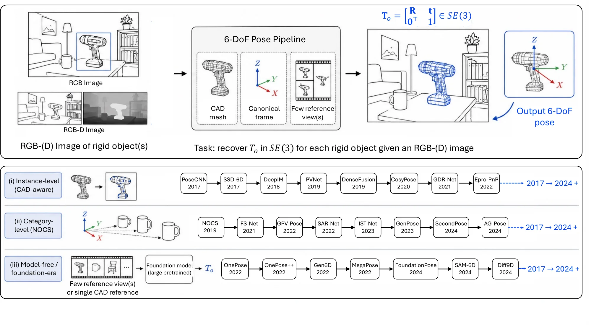
Instance-Level 6-DoF: CAD-Aware Pipelines. With a mesh of each target object available, pose estimation becomes alignment of the mesh with image evidence, and synthetic renderings of the CAD models are the main training signal. PoseCNN [737] set the modern baseline by regressing an object’s image-space center and a quaternion rotation with a CNN, and introduced the YCB-Video benchmark. A second family decouples the network from the geometric solver by predicting projections of sparse 3D keypoints and solving PnP with RANSAC; PVNet [738] votes per pixel for each keypoint, which makes it robust to occlusion, while SSD-6D [739] folds a discretized viewpoint classification into a detector and skips PnP entirely. A third family regresses dense object coordinates instead of sparse keypoints: DenseFusion [740] fuses RGB-D features per pixel for iterative refinement, GDR-Net [741] couples dense coordinate regression with a geometry-guided PnP layer, ZebraPose [742] encodes the surface with a coarse-to-fine binary code, and SurfEmb [743] learns continuous correspondence distributions that stay robust under symmetry and occlusion; EPro-PnP [744] replaces the non-differentiable PnP solver with a probabilistic surrogate so the whole pipeline trains end to end. A fourth family refines by render-and-compare: DeepIM [745] iteratively minimizes the residual between a rendered CAD view and the image, and CosyPose [746] extends this to consistent multi-view, multi-object refinement and led the BOP 2020 leaderboard. The same machinery reaches far from the tabletop, for example spacecraft pose under extreme scale variation [747].
Category-Level 6-DoF + Size: Canonical Frame Recovery. Without a per-instance mesh but with a category that admits a canonical frame, pose is recovered up to that frame together with absolute scale, a 9-DoF prediction. NOCS [710] introduced the formulation, mapping every instance of a category into a Normalized Object Coordinate Space and regressing dense correspondences there; its REAL275 benchmark is the standard category-level evaluation. Later work re-parameterizes the problem: FS-Net [748] decouples rotation, translation, and size and speeds up inference through a shape-based pathway, GPV-Pose [749] grounds rotation in geometry-guided point-wise voting, SAR-Net [750] recovers a deformed shape prior alongside pose to handle intra-class variation, and IST-Net [751] drops the shape prior and learns the canonical transformation implicitly. SecondPose [752] and AG-Pose [753] import DINOv2 semantics and instance-adaptive keypoints for further gains on REAL275, and GenPose [754] casts category-level pose as score-based diffusion sampling, the precursor of the 9-DoF diffusion model below. The family’s standing assumption, that a meaningful canonical frame exists per category, holds for mugs and cameras but fails for heterogeneous semantic groupings, which motivates the model-free line.
Model-Free / Novel-Object Pose: Foundation-Model Era. The largest recent shift is away from per-object and per-category training toward objects first seen at test time, given only a few reference images or a CAD model. From a short reference video, OnePose [755] triangulates a feature point cloud and matches test queries against it, OnePose++ [756] removes the dependence on repeatable keypoints with a dense-matching front end, and Gen6D [757] unifies detection, viewpoint selection, and refinement without per-object fine-tuning. From a CAD model alone, MegaPose [758] trains render-and-compare on millions of synthetic objects and transfers zero-shot, FoundationPose [759] consolidates model-based and model-free operation under large-scale synthetic pretraining and leads the BOP novel-object track, GigaPose [760] cuts the cost of render-and-compare by sampling templates in a two-DoF rotation space and recovering the remaining parameters from a single patch correspondence, and SAM-6D [761] uses the Segment Anything Model [138] as a zero-shot detection front end before learned pose matching. A further sub-line drops pose-specific training altogether and matches frozen foundation features: FoundPose [762] establishes 2D–3D correspondences between DINOv2 patch descriptors of the query and pre-rendered templates, and FreeZe [763] fuses frozen 3D geometric descriptors with 2D foundation features and recovers pose by RANSAC registration; a FreeZe variant took first place for unseen-object localization and detection in the BOP Challenge 2024 [764], overtaking the render-and-compare line. Diff9D [765] reformulates 9-DoF category-level pose as diffusion sampling, the object-pose instance of the diffusion-as-perception pattern seen for depth and normals, which yields calibrated multi-hypothesis predictions (natural for symmetric objects) at the cost of latency. The foundation-model line has thus largely dissolved the instance-versus-category-versus-model-free distinction; the active question is how cheap the per-test-object supervision can become.
Sensing Modalities. Across these axes, the input modality fixes which supervisory signals exist and which symmetries can be resolved. RGB-only pipelines [737, 738, 741, 744, 755] suit mobile and AR deployment but face scale–depth ambiguity on texture-poor objects; RGB-D fusion (DenseFusion [740], CosyPose [746] with depth refinement, FoundationPose [759]) is substantially more accurate on BOP at the cost of a depth sensor; depth-only methods are rare but remain competitive on highly symmetric objects where shading carries little rotational evidence. Monocular depth foundation models (§6.2.1) are increasingly used as plug-in depth providers at inference, which narrows the RGB / RGB-D gap without an active sensor.
6.2.5.3Datasets and Metrics#
Table 6.15 lists the recurring benchmarks. Instance-level evaluation grew from LINEMOD [766], the texture-rich entry point that introduced the ADD metric, through its occlusion-heavy re-annotation LINEMOD-Occluded [767], which modern methods report as the more informative of the two, to the video setting of YCB-Video [737] and the texture-less, symmetric industrial parts of T-LESS [768], where symmetry handling decides the ranking; HomebrewedDB [769] serves as an out-of-distribution test for methods trained on the BOP core data, and SPEED [770] stretches the task to spacecraft under scale and illumination ranges no tabletop set covers. NOCS-REAL275 with its synthetic companion CAMERA [710] is the category-level standard. The BOP Challenge [771, 772, 773] consolidates the instance-level datasets under one protocol and has been the field’s headline leaderboard since 2017; its 2023 edition separates a classical CAD-known track from a novel-object track, formalizing the model-free shift. Modern papers report at minimum on LINEMOD-Occluded, YCB-Video, and a BOP-core subset, novel-object methods add the BOP unseen-object track, and category-level methods center on REAL275.
| Dataset | Year | Setting | Objects | Frames | Role |
| LINEMOD [766] | 2012 | Instance, textured household, RGB-D | 15 | 1.2K / object | Entry benchmark; introduced ADD |
| LINEMOD-Occluded [767] | 2014 | Instance, heavy mutual occlusion | 8 | re-annotated LM scene | Occlusion stress test |
| YCB-Video [737] | 2017 | Instance, RGB-D video, moving camera | 21 | 133K | Sequential pose and tracking |
| T-LESS [768] | 2017 | Instance, texture-less, symmetric industrial parts | 30 | – | Symmetry / texture-poor stress test |
| HomebrewedDB [769] | 2019 | Instance, household scenes | – | – | Out-of-distribution generalization |
| NOCS-REAL275 (+CAMERA) [710] | 2019 | Category-level 9-DoF, RGB-D | 6 categories | 8K real (+ synthetic) | Category-level standard |
| SPEED [770] | 2019 | Spacecraft, extreme scale and lighting | 1 | – | Beyond-tabletop deployment |
| BOP Challenge [771, 772, 773] | 2018– | Unified protocol over LM-O, T-LESS, YCB-V, ITODD, IC-BIN, TUD-L, HB, HOPE | – | – | Headline leaderboard; novel-object track since 2023 |
Each metric answers to a particular failure mode of pose error, and the symmetry-aware variants exist because many objects admit several valid poses. The Average Distance of Model Points (ADD) is the standard for asymmetric objects: with predicted pose , ground truth , and mesh vertices ,
| (6.30) |
and a pose counts as correct when for object diameter , the ADD-0.1d threshold introduced with LINEMOD [766]. For symmetric objects ADD-S replaces direct vertex correspondence with nearest-neighbor matching,
| (6.31) |
under the same threshold; the two are reported together so that symmetric and asymmetric objects are diagnosed separately. For AR overlay the relevant error is in image space, so the 2D projection error averages the pixel distance between mesh vertices projected under the two poses, with 5 px as the usual threshold. Category-level evaluation on REAL275 counts a prediction correct when
| (6.32) |
and adds 3D box IoU at and to score pose and size jointly. The BOP Challenge [771] averages recall over three symmetry-aware errors, each thresholded at several operating points: the Visible Surface Discrepancy (VSD), which scores only the visible object surface and is therefore robust to occlusion, the Maximum Symmetry-aware Surface Distance (MSSD), the worst-case surface deviation over all valid symmetries, and its image-space analogue MSPD,
| (6.33) |
averaged over the BOP core datasets. ADD and ADD-S remain the default for LINEMOD-style instance-level work, BOP-AR for cross-dataset comparison, and projection error for AR; the metrics persist side by side because no single norm captures both strict pose error and the equivalence-class structure that VSD and MSSD make explicit.
| Method | Family | Modality | Train assumption | Year | ADD-0.1d | BOP-AR |
| PoseCNN [737] | Instance / direct | RGB | per-object | 2017 | 24.9 | – |
| PVNet [738] | Instance / keypoint+PnP | RGB | per-object | 2019 | 40.8 | – |
| GDR-Net [741] | Instance / coord. reg. | RGB | per-object | 2021 | 62.2 | – |
| CosyPose [746] | Instance / refinement | RGB | per-object | 2020 | – | 63.3 |
| SurfEmb [743] | Instance / dense corr. | RGB-D | per-object | 2022 | – | 75.8 |
| MegaPose [758] | Model-free / render&comp. | RGB-D | cross-object | 2022 | – | 58.3 |
| FoundationPose [759] | Model-free / found. | RGB-D | cross-object | 2024 | – | 78.8 |
Table 6.16 reports LINEMOD-Occluded, the most widely used instance-level benchmark under the BOP protocol. Among RGB methods scored by ADD(-S)-0.1d, explicit geometry steadily closes the gap over direct regression: PoseCNN’s 24.9 rises to 40.8 with per-pixel keypoint voting (PVNet) and to 62.2 with geometry-guided dense coordinate regression (GDR-Net). On the symmetry-aware BOP-AR, the render-and-compare CosyPose (63.3) and the dense-correspondence SurfEmb (75.8) are now matched or exceeded by model-free systems with no per-object training, FoundationPose reaching 78.8 against MegaPose’s earlier 58.3; this is the 2023–2024 shift that made novel-object pose a deployment target rather than a research curiosity. The gap between the two families is widest on the symmetric objects of T-LESS, where losses that model symmetry (BOP-AR-aware objectives, ADD-S optimization) generalize better than those assuming a single asymmetric pose.
6.2.5.4Challenges#
The onboarding bottleneck has shifted from pose to detection. Moving to novel objects relocated the limiting stage rather than removing it. On the BOP Challenge 2024 [764], 6-DoF localization of unseen objects has nearly caught up with the seen-object regime (the strongest training-free entry, a FreeZe variant [763], trails the best seen-object method by a few points of average recall), whereas detection of unseen objects still lags its seen-object counterpart by roughly a third and is now the largest error source in the novel-object stack. The open problem is zero-shot detection and segmentation of a never-seen instance in clutter, together with the cost of onboarding it: BOP 2024 added a track in which an object is registered from a short reference video, Any6D [774] registers from a single RGB-D anchor image, and how few views, or whether a single image or a text prompt, suffice is the defining frontier question. The same challenge pivoted toward high-resolution AR/VR headset recordings, a signal that the benchmark-realism gap, including articulated and deformable objects, open-vocabulary targets named rather than modeled (POPE [775]), and egocentric capture, is now a first-order concern.
Absolute metric scale remains ambiguous for model-free targets. The true size of an unseen object is under-determined from RGB alone, since scale and depth trade off along the viewing ray. Category-level 9-DoF methods absorb this by regressing size in a canonical frame [710], and model-free systems lean on a depth sensor or a known CAD extent; when neither is available, scale is the residual unknown separating a plausible pose from a usable one, which Any6D [774] makes explicit by coupling pose recovery with scale alignment, and monocular depth priors inherit the affine ambiguity of §6.2.1.
Accuracy trades sharply against latency. The methods that top the novel-object leaderboard are the least suited to closed-loop use: on BOP 2024 [764] the most accurate unseen-object method runs in tens of seconds per image, close to an order of magnitude slower than both the fastest seen-object pipelines and the practical sub-second entries, which buy speed with accuracy. Heavy segmentation, render-and-compare, and diffusion priors (Diff9D [765]) are the cause, which is why one-correspondence template matching (GigaPose [760]), distillation, and selective invocation of expensive components have become load-bearing for robotic and AR loops at frame rate.
Symmetry and geometric ambiguity are irreducible. Symmetric and texture-less parts of the kind that fill T-LESS [768] admit a continuous or discrete family of photometrically indistinguishable poses, and any loss assuming a unique target diverges on them; transparent and specular surfaces violate the brightness-constancy and depth-sensing assumptions behind correspondence and RGB-D fusion; rotation parameterization adds degeneracies that continuous 6D or axis-angle encodings reduce but do not remove; and heavy occlusion, the regime of LINEMOD-Occluded [767], starves the estimator of the evidence needed to resolve any of them. Generative multi-hypothesis pose (Diff9D [765]) predicts a distribution instead of a point, but turning that distribution into a calibrated confidence a planner can trust in safety-critical manipulation and driving is still largely unaddressed.
Across these problems, pose pipelines increasingly consume foundation-model priors as plug-in modules (promptable segmentation for zero-shot detection, monocular depth for inference-time geometry) rather than training pose-specific backbones, and the boundary between pose estimation, 6-DoF tracking, and neural reconstruction is dissolving, as FoundationPose [759] folds estimation and tracking into one loop and the reconstruction discussion of Chapter 8 pursues further. Promptable, real-time, uncertainty-aware pose is the target the next generation of methods converges on.