12.2.1Introduction#
A physical system is a field over space; a molecule or a material is a three-dimensional arrangement of atoms together with an electronic field over that arrangement; a protein, a cell, or a tissue is a three-dimensional structure whose function follows from its form. In every case the scientific quantity of interest, whether an energy, a reaction rate, a biological function, or a material property, is a function of spatial structure under strict symmetry constraints, so that understanding nature is to a large degree a problem of recovering and reasoning about that structure.
The geometric representations of Chapter 4 and the reconstruction and generation of Chapter 8 reappear here specialized to data that obey physical law: to fields constrained by differential equations, to atomic systems constrained by Euclidean and permutation symmetry, and to biomolecules whose geometry determines their function. A single capability triad recurs inside every domain and gives the section its spine: spatial representation and reconstruction recovers a continuous field or a 3D structure from sparse, indirect, and noisy measurements; dynamics, simulation, and law discovery learns how that structure evolves and what governs it; and design, discovery, and control either generates new structure or inverts observations for hidden causes. The third leg reads as discovery and control in physics and as generative design in chemistry and life science.
The section is organized by scientific domain (physics, chemistry, and life science); the earth and environmental sciences are treated at geographic scale in the GeoAI of §11.2, the clinical, patient-scale counterpart of the life-science material in §12.1, and the generic digital twin in §11.1. Figure 12.5 previews the section as a cross-scale map in which the three domains share the same vertical triad, and Table 12.2 collects a representative benchmark for each capability.
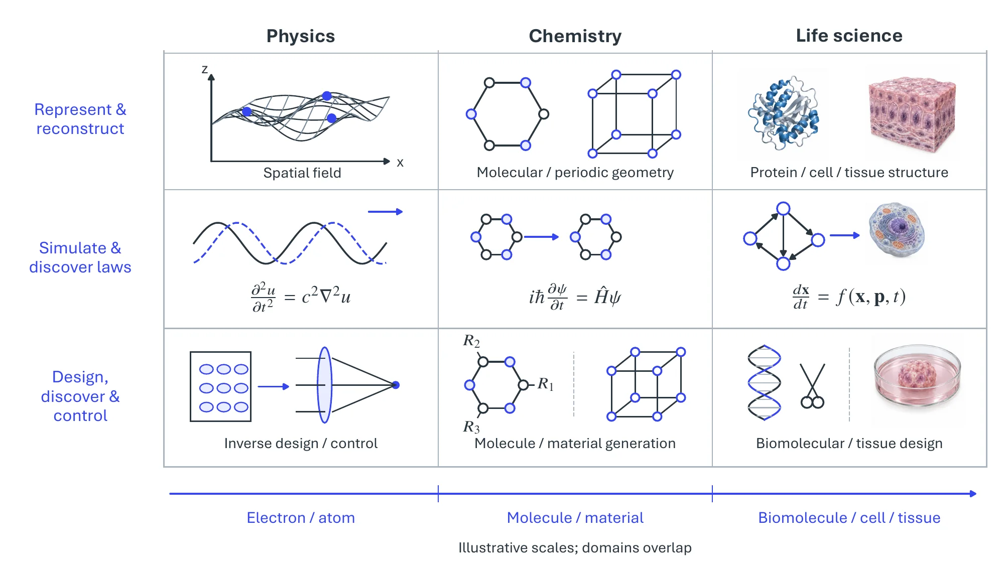
12.2.2Physics#
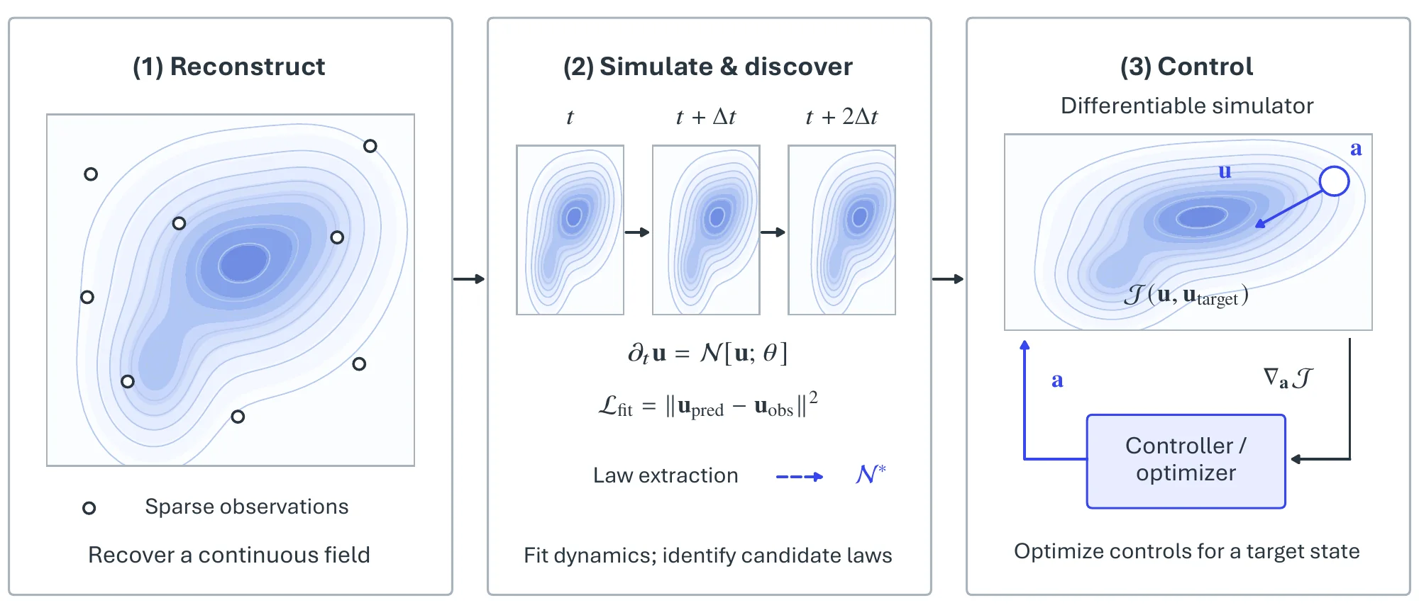
Spatial intelligence in physics constructs spatial structure and discovers the laws that govern its motion, and it earns its place where first-principles solvers are too costly or the governing equations are unknown: fields are reconstructed from limited observations, their dynamics are modeled and their laws discovered, and the systems are optimized and controlled. Figure 12.6 previews this progression from a sparsely observed field to a learned dynamical rollout and a differentiable-control loop.
12.2.2.1Spatial Representation and Reconstruction#
Many key quantities in physical systems are available only through sparse and noisy observations, and representation and reconstruction recover continuous spatial fields from such data, the input to law discovery and control. Embedding physical priors such as governing partial differential equations and symmetry constraints keeps these reconstructions physically consistent in low-data regimes.
A classical task is physical field reconstruction, which aims to recover continuous physical fields such as temperature, pressure, and velocity from sparse sensor readings or boundary measurements; the central challenge lies in ensuring the physical plausibility of the solution under the ill-posed conditions caused by insufficient observations. Physics-informed neural networks are a classical approach for this task [2680], embedding partial differential equations such as the Navier–Stokes equations as soft constraints in the loss function and computing physical residuals via automatic differentiation, which enables accurate reconstruction of fluid and thermal fields in data-scarce settings; the same networks serve as real-time surrogates in digital twins (§11.1). Neural fields implicitly represent continuous physical fields by using coordinate-based networks that map spatial locations to physical quantities. Sitzmann et al. [2884] proposed SIREN, which employs periodic activation functions to capture high-frequency spatial details with high fidelity and has been applied to solving Poisson equations and reconstructing wave fields. The general machinery of coordinate-based neural representation is developed in Chapter 8.
Inverse scattering aims to infer the internal structure or material parameters of an object from measured wave-scattering data, and it remains a canonical ill-posed problem in electromagnetics and acoustics [2885]. Wei and Chen proposed deep-learning schemes [2886] for full-wave nonlinear inverse scattering that directly invert dielectric-permittivity profiles from scattered fields, thereby moving beyond linearized Born-type approximations in practical reconstructions. SwitchNet [2887] introduced a unified neural architecture that learns both the forward map from scatterers to scattered fields and the inverse map from measurements to scatterer profiles, using a switching layer that exploits low-rank structure to reduce model complexity and facilitate training. Physics-guided losses that inject multiple-scattering near-field priors into the objective further improve robustness.
12.2.2.2Dynamics, Simulation, and Law Discovery#
Law discovery aims to learn the generative structures or explicit laws that govern the evolution of physical systems from observational data, emphasizing the automatic extraction of conservation laws, symmetries, and interpretable mechanisms beyond accurate prediction. Hamiltonian Neural Networks [2888] directly learn the Hamiltonian of a system, thereby enforcing energy conservation and symplectic structure at the model level and providing a principled foundation for interpretable dynamical modeling. Lagrangian Neural Networks [2889] parameterize arbitrary Lagrangians with neural networks, learning energy conserving dynamics without canonical coordinates, as validated on the double pendulum and a relativistic particle. Cranmer et al. [2890] combine graph networks with symbolic regression on their internal representations, recovering known force laws and Hamiltonians, and applying the approach to cosmology. The SINDy algorithm [2891] employs sparse regression to identify governing differential equations directly from time-series data, enabling data-driven discovery of interpretable physical laws.
Efficient physical solvers focus on predicting the spatio-temporal evolution of physical systems under known governing equations or interaction rules, with the goal of achieving fast and scalable computation while preserving physical consistency beyond the limits of traditional numerical methods. The Fourier Neural Operator [2892] learns mappings between function spaces rather than individual discretized instances, enabling trained models to predict the evolution of partial differential equations at arbitrary spatial resolutions without relying on a fixed computational grid. DeepONet [2893], grounded in the universal approximation theorem for operators, learns nonlinear mappings from input functions to output functions and thereby approximates the solution operators that govern physical systems. Interaction Networks [1201] introduced the relational reasoning architecture that learns physical interactions between objects, laying the foundation for graph-based physical simulation. The Graph Network Simulator [2894] employs graph neural networks to model spatial interactions among particles or objects, achieving high-fidelity simulations of fluids, rigid bodies, and deformable materials, and MeshGraphNets [2895] extend graph-based models to unstructured meshes, allowing efficient simulation of continuum mechanics on irregular geometries. For the classical challenge of turbulence modeling, Mohan et al. [2896] proposed spatio-temporal deep-learning models with physics-informed diagnostics that improve the prediction accuracy of three-dimensional turbulent flows, and Lusch et al. [2897] developed a deep-learning framework for universal linear embeddings of nonlinear dynamics, enabling low-dimensional representations and long-term prediction of nonlinear fluid systems. Neural representations of the many-body wavefunction are treated with electronic structure in the chemistry subsection.
12.2.2.3Control and Optimization#
Optimization and control in physical systems seek optimal trajectories, shapes, or control policies under governing physical laws and environmental constraints. Differentiable physics formulates physical simulators as differentiable operators, enabling gradient-based optimization over control inputs, design variables, and physical parameters, and providing a unified framework for optimal control, system identification, and design. Neural Ordinary Differential Equations [2898] provide a differentiable formulation of continuous-time dynamical systems by parameterizing the vector field with a neural network and enabling gradient computation through adjoint sensitivity analysis, serving as a flexible building block for learning and control in continuous time. ChainQueen [2899] demonstrates differentiable simulation of soft and deformable bodies based on the moving least squares material point method, enabling gradient-based optimization in high-degree-of-freedom systems with contact and supporting applications in soft-robot control and co-design. DiffTaichi [2678] generalizes this paradigm through a differentiable programming framework for high-performance physical simulation, allowing efficient construction of differentiable solvers and gradient-driven optimization for fluid control, shape optimization, and material-parameter estimation; the same tools calibrate digital twins (§11.1). In practice, a mature software substrate of differentiable and physics-informed libraries, such as DeepXDE1 and NVIDIA Modulus2 for operator and PINN training, and JAX-MD3 and DeePMD-kit4 for differentiable and learned-potential molecular dynamics, turns this triad into runnable physics.
12.2.3Chemistry#
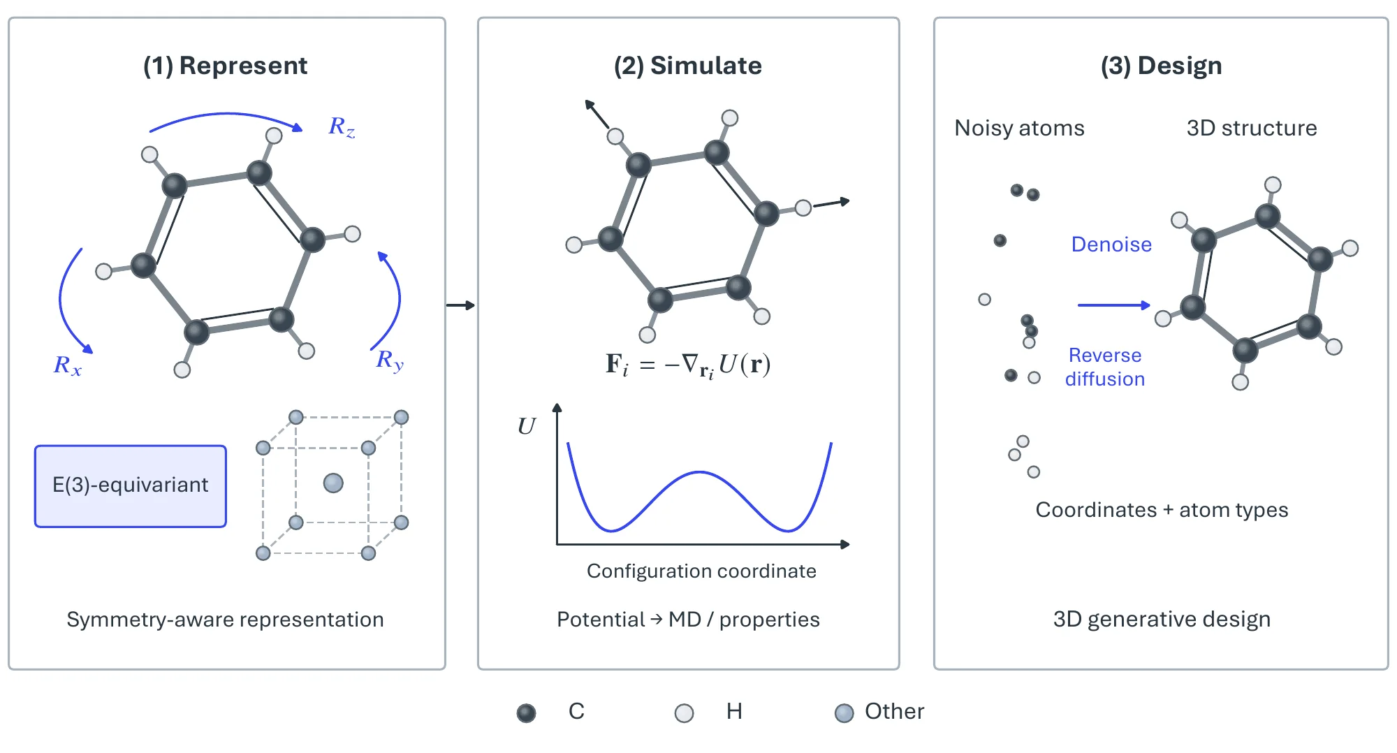
Chemistry is intrinsically spatial: a molecule or a material is a three-dimensional arrangement of atoms together with an electronic field over it, and its behavior, whether energy, reactivity, or a bulk property, is a function of that geometry under strict symmetry. Physical observables must be invariant or equivariant to the Euclidean group of rotations, translations, and reflections and to permutations of identical atoms; for crystalline solids they must also respect periodic lattice symmetry, and for electrons they must obey antisymmetry under exchange. Spatial intelligence in chemistry is therefore largely the art of building these symmetries into models that represent atomic and electronic structure, simulate its dynamics, and generate new structure under chemical feasibility. Figure 12.7 previews this triad from an equivariant representation of a 3D structure to a learned-potential simulation and a 3D generative design.
12.2.3.1Spatial Representation and Reconstruction#
The central representational problem of chemistry is to map a 3D atomic geometry to energies, forces, and properties while respecting symmetry, and successive representations have captured progressively more of that geometry. Geometry-grounded potentials. The Behler–Parrinello neural network potential founded the area by decomposing the total energy into atomic contributions computed from rotation-, translation-, and permutation-invariant symmetry functions of each atom’s local environment [2900]. SchNet [2901] replaced hand-designed descriptors with continuous-filter convolutions over interatomic distances, giving a smooth invariant representation for energy and force prediction, while DimeNet [2902] added directional message passing that encodes bond angles through spherical harmonics, moving beyond pairwise distances to angular structure, and PaiNN [2903] extended message passing to rotationally equivariant vector features for tensorial properties and spectra. The Deep Potential model [2904] preserves all natural symmetries at linear cost, and the ANI potentials [2905] demonstrated transferable organic-chemistry accuracy at force-field cost. Equivariant interatomic potentials. The decisive recent step was to carry geometric tensors, not merely invariant scalars, through the network. NequIP [1380] introduced E(3)-equivariant convolutions over geometric tensors and achieved striking data efficiency, often requiring orders of magnitude less training data; Allegro [2906] made the representation strictly local and thereby scalable to 100 million atoms, and MACE [1381] used higher body-order equivariant messages to reach high accuracy in only two message-passing layers. A further shift is from per-system fits to universal potentials that span the periodic table: M3GNet [2907] couples a graph network with explicit three-body interactions trained on materials relaxations, and CHGNet [2908] augments the 3D-structure graph with atomic magnetic moments to capture electronic degrees of freedom alongside geometry. These equivariant backbones share machinery with the geometric representations of Chapter 4. Neural electronic structure. At the quantum scale the spatial object is the many-electron wavefunction itself. Neural quantum states parameterize that wavefunction with a neural network over spin configurations [2909], and deep variational ansätze such as FermiNet [2910] and PauliNet [2911] operate directly on 3D electron coordinates while enforcing exact antisymmetry, solving the electronic Schrödinger equation to chemical accuracy from nuclear positions alone.
12.2.3.2Dynamics, Simulation, and Property Prediction#
The potentials of the previous thread are also the simulators: once a model maps a 3D configuration to energies and forces, it drives molecular dynamics at a fraction of the cost of first-principles calculation, and the same representations predict quantum properties such as energies, dipoles, and frontier-orbital gaps directly from coordinates. The gradient-domain machine-learning force field made this explicit by exploiting energy conservation and the geometry of conformations, and it established the widely used MD17 trajectory benchmark of energies and forces for small molecules [2912]. Heterogeneous catalysis pushes the same energy-and-force prediction task to a far larger and more diverse chemical space, spanning many combinations of metal surfaces and adsorbates. GemNet-OC [2913] extends directional message passing to this setting, delivering accurate energies and forces across the surfaces and adsorbates of the Open Catalyst datasets. In parallel, structure-to-property prediction is standardized on QM9 [1379], a dataset of roughly 134,000 small organic molecules with density-functional geometries and quantum properties, on which the equivariant networks above are routinely evaluated by the mean absolute error of predicted properties. This ecosystem rests on open toolkits, including the equivariant-network library e3nn5, the atomistic-simulation environment ASE6, and the quantum-chemistry package PySCF7, together with universal-potential foundation models such as MACE-MP, and on reference corpora such as the Materials Project [2914], the Open Catalyst dataset [2915], and the MoleculeNet benchmark suite [2916].
12.2.3.3Generation and Inverse Design#
The inverse of property prediction is design: generating new 3D structures that satisfy desired properties under chemical feasibility, by sampling on the appropriate geometric manifold rather than enumerating candidates. G-SchNet [2917] autoregressively places atoms in 3D Euclidean space with each placement respecting the rotational invariance and local symmetry of those already placed, the first strong 3D-native generator. Diffusion models then became the dominant paradigm: the equivariant diffusion model [2918] jointly denoises atom coordinates and types under E(3) equivariance, GeoDiff [2919] generates conformers from the molecular graph through roto-translation-equivariant Markov kernels that induce an invariant distribution, and torsional diffusion [2920] restricts the process to the hypertorus of torsion angles, the true intrinsic conformational degrees of freedom, achieving state-of-the-art conformer quality on GEOM-Drugs [2921] at a fraction of the cost. For crystalline materials, CDVAE [2922] generates stable structures under periodicity and SE(3) invariance and supports inverse design by optimizing target properties in latent space. The line has since moved to diffusion directly on the periodic structure: DiffCSP [2923] jointly denoises lattice and fractional coordinates under periodic equivariance for crystal structure prediction, and MatterGen [2924] scales this into a property-conditioned foundation model for inorganic materials design, with generated candidates validated by experimental synthesis. The general diffusion machinery underlying these models is developed in Chapter 8; what is chemistry-specific is the constraint manifold (valence and bonding feasibility, energy-minimum geometries, lattice periodicity) on which generation must take place.
12.2.4Life Science#
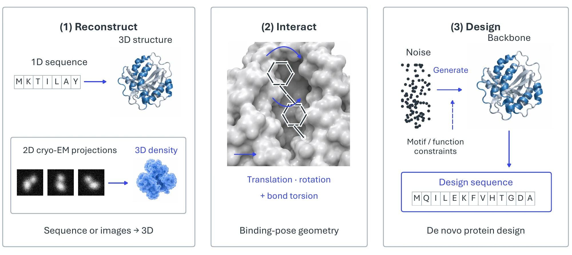
At the molecular, cellular, and tissue scale of basic biology the object of interest is again a three-dimensional structure: a protein fold, a molecular complex, a spatial map of gene expression, or the wiring of a neural circuit, and in each case function follows from spatial form. Spatial intelligence here recovers that structure from indirect measurement, models how biomolecules interact and move, and designs new structure. Figure 12.8 previews the triad from structure recovery through interaction modeling to generative design.
12.2.4.1Spatial Representation and Reconstruction#
The defining achievement of spatial intelligence in biology is the recovery of 3D structure from indirect signals. Protein structure prediction maps a one-dimensional sequence to a three-dimensional fold. The original AlphaFold predicted inter-residue distance distributions as a learned potential to fold the chain [2925], and AlphaFold2 [2926] reached near-experimental accuracy through an end-to-end architecture that reasons explicitly over residue frames and pairwise geometry, the exemplar of spatial intelligence in the natural sciences. AlphaFold3 [2927] generalized this to the joint structure of proteins, nucleic acids, and small molecules through a diffusion decoder; RoseTTAFold [2928] let one-dimensional, two-dimensional, and three-dimensional information flow between tracks, and ESMFold [2929] showed that atomic-level structure emerges from a protein language model without explicit alignments, enabling metagenomic-scale folding. Cryo-electron microscopy solves the inverse problem of reconstructing a 3D density map from many noisy 2D projections. RELION cast this as Bayesian refinement [2930], CryoSPARC enabled rapid ab-initio reconstruction without a starting model [2931], and cryoDRGN used a coordinate-based neural decoder to reconstruct continuous distributions of conformations and thereby resolve molecular heterogeneity and motion [2932]. Spatial transcriptomics places gene expression back into tissue space. The founding barcoded-array assay preserved the positional information of the transcriptome in tissue sections [2933]; Tangram learns a spatial mapping that aligns dissociated single cells onto a spatial reference [2934], and novoSpaRc reconstructs spatial arrangement from expression alone through optimal transport, assuming that expression-similar cells lie physically close [2935]. Connectomics reconstructs neural wiring from electron-microscopy volumes, where flood-filling networks iteratively trace the 3D morphology of individual neurites through the volume [2936].
12.2.4.2Dynamics, Simulation, and Interaction#
Beyond static structure, spatial intelligence models how biomolecules bind and interact. Molecular docking predicts the 3D pose in which a ligand binds a protein, and recent methods treat it as a geometric problem on the natural manifold of poses. DiffDock [2937] formulates docking as diffusion over the product space of ligand translation, rotation, and torsion, sampling binding poses in their intrinsic degrees of freedom, while EquiBind [2938] regresses the binding location and pose in a single shot using an SE(3)-equivariant network whose equivariance encodes the rotational and translational symmetry of the binding geometry. Protein–protein and complex geometry is predicted by extending folding models to multiple chains [2939], and AlphaFold3 above provides a generative alternative for protein–ligand and protein–nucleic-acid complexes. The dynamics of biomolecules in turn rest on the learned interatomic potentials of the chemistry subsection, which accelerate the molecular dynamics that sample conformational change.
12.2.4.3Generation and Design#
The generative leg designs new 3D biological structure. RFdiffusion [2940] adapts structure-denoising diffusion to generate novel protein backbones conditioned on functional and geometric constraints such as motif scaffolding, binders, and symmetric assemblies, and ProteinMPNN [2941] solves the inverse-folding problem of designing an amino-acid sequence that folds into a given 3D backbone, the standard partner to backbone generation. Chroma [2942] couples equivariant graph networks with a diffusion process to sample novel all-atom structures and sequences steerable toward desired properties, illuminating regions of protein space never explored by evolution. As in chemistry, the underlying diffusion machinery is that of Chapter 8; what is biology-specific is that the generated geometry must be foldable and functional, which is why design is paired with structure prediction and, ultimately, wet-lab validation. The field is supported by open infrastructure, including the AlphaFold Protein Structure Database and AlphaFold3 server8, the ESM Metagenomic Atlas9, and the open-source folding stack OpenFold10, together with reference corpora such as the Protein Data Bank, the CASP blind-assessment benchmark [2943], and the PDBBind docking benchmark [2944].
| Domain | Capability | Benchmark / dataset | Representative method | Headline metric |
| Physics | PDE surrogate | Navier–Stokes / Darcy flow | FNO [2892] | relative error |
| Physics | Particle dynamics | Learning-to-Simulate suite (Water / Sand / Goop) | GNS [2894] | rollout MSE |
| Chemistry | Property prediction | QM9 [1379] | DimeNet [2902] | property MAE |
| Chemistry | Force field | MD17 [2912] | NequIP [1380] | energy / force MAE |
| Chemistry | Catalysis | Open Catalyst [2915] | GemNet-OC [2913] | energy / force MAE |
| Chemistry | Conformer generation | GEOM-Drugs [2921] | torsional diffusion [2920] | coverage / matching RMSD |
| Life science | Protein folding | CASP [2943] | AlphaFold2 [2926] | GDT-TS |
| Life science | Docking | PDBBind [2944] | DiffDock [2937] | top-1 RMSD Å (%) |
| Life science | Cryo-EM heterogeneity | EMPIAR single-particle datasets | cryoDRGN [2932] | resolution (FSC) |
| Life science | Protein design | Motif-scaffolding / binder design | RFdiffusion [2940] | in-silico design success rate |
12.2.5Challenges#
A learned model of nature has to respect the symmetries and conservation laws of its domain and remain correct outside the data it was fitted to. The six problems below follow from that requirement: how to build symmetry in, how to bridge scales, how to solve ill-posed inverse problems, how to learn from scarce and expensive labels, how to generalize to genuinely new systems, and how to make predictions physically consistent and trustworthy.
Symmetry and Equivariance. Physical observables are constrained by symmetry: Euclidean invariance and equivariance, permutation of identical particles, antisymmetry of electrons, and periodicity of crystals. Whether to build these symmetries into the architecture or to learn them from data is the central design tension, trading the cheaper but less expressive invariant features [2901] against the richer but costlier equivariant tensor features [1380], and it recurs from interatomic potentials to protein structure.
Extreme Multi-Scale Structure. Spatial structure in nature spans many orders of magnitude, from electrons and atoms to molecules and materials, and from biomolecules through cells to tissue. Learned potentials now reach a hundred million atoms [2906], still far below cellular scale; no single representation natively bridges electronic-structure accuracy and mesoscale reachability, and the handoffs between scales, through coarse-graining or learned-potential dynamics, are lossy and remain only partially solved.
Ill-Posed Inverse Problems. Much of natural science is an inverse problem in which a high-dimensional spatial field must be recovered from sparse, indirect, and noisy measurements: field reconstruction from a few sensors, inverse scattering [2886], and the recovery of 3D density from 2D cryo-electron-microscopy projections [2932] all share this under-determined character and demand strong learned priors to yield a unique and physical solution.
Data Scarcity and the Cost of Ground Truth. High-fidelity labels are expensive: accurate energies and forces require costly quantum-chemistry calculations, which is why force-field benchmarks such as MD17 cover only small molecules [2912], and validated 3D biological structures require slow experiments, so the space of trustworthy training data is small relative to the space of possible systems. This drives the field’s emphasis on data efficiency, multi-fidelity learning, and physics-guided objectives.
Generalization Beyond the Training Distribution. Models must extrapolate to unseen chemistry, novel protein folds, off-equilibrium and reactive geometries, and configurations far from those they were trained on. Discovery is by definition out of distribution, so leaderboard accuracy says little about it; this is why generative materials design is now judged by whether its candidates can actually be synthesized [2924].
Physical Consistency and Trust. Predictions that violate conservation laws or come without calibrated uncertainty cannot support a scientific conclusion. Building conservation into the model, as Hamiltonian networks do for energy [2888], and quantifying confidence are what let a learned model extend the scientific record rather than interpolate it.
- https://github.com/lululxvi/deepxde↩
- https://developer.nvidia.com/modulus↩
- https://github.com/jax-md/jax-md↩
- https://github.com/deepmodeling/deepmd-kit↩
- https://e3nn.org/↩
- https://wiki.fysik.dtu.dk/ase/↩
- https://pyscf.org/↩
- https://alphafoldserver.com/↩
- https://esmatlas.com/↩
- https://github.com/aqlaboratory/openfold↩