Before space can be measured or organized; its contents must be named. Spatial entity recognition is that entry point: it answers what is present, and every later geometric and relational step builds on the entities it names. Recognition operates at several granularities, and the section is ordered accordingly: detecting discrete object instances, delineating dense regions of pixels or points by segmentation, pinning down sparse keypoints and landmarks, and finally assigning a holistic scene label. What unites them is that they recover identity and category, not yet geometry; where each entity sits and how it is oriented is taken up next.
6.1.1Object Detection#
6.1.1.1Task Definition#
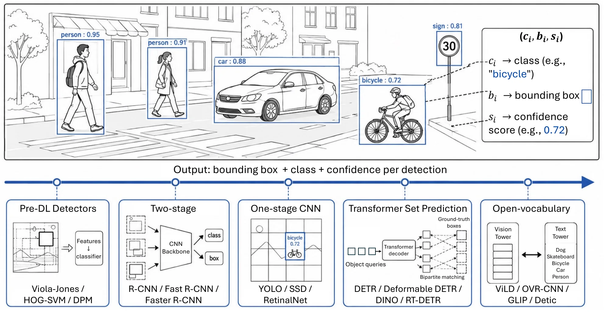
Given a 2D image , 2D object detection identifies instances of predefined object classes and localizes each one in the image plane. The output is a set of detections
| (6.1) |
where is the predicted class, a 2D bounding box (center and size, or corner coordinates), and a confidence score. In short, the task answers what objects are where. Figure 6.1 summarizes the 2D task and its detector families.
3D object detection keeps the same set-of-detections output but places each box in metric 3D space. The input is a LiDAR point cloud with (often with an intensity channel), one or more calibrated images, or both, and each box becomes
| (6.2) |
a 3D center, the physical length, width, and height, and a heading angle about the vertical axis; indoor benchmarks often use axis-aligned boxes and drop . Because the box is expressed in the sensor or ego frame rather than the image plane, a 3D detection already carries metric position and heading, which is why driving and robotics stacks consume it directly.
6.1.1.2Methodology#
Before Deep Learning. Early detectors [401] ran a sliding window over multi-scale image pyramids and classified each candidate region with hand-crafted features and shallow models. Viola–Jones [402] combined Haar-like features with an AdaBoost cascade for real-time face detection; HOG features with linear SVMs [403] became the standard pipeline for pedestrians and generic objects; and deformable part-based models (DPMs) [404] represented an object as parts connected by deformable constraints. Manual feature design, dense-window evaluation, and limited robustness to pose, scale, and occlusion capped this line and motivated the move to learned features.
Two-stage Detectors. R-CNN [126] first generates category-independent region proposals and then classifies each with a CNN, a large accuracy gain over hand-crafted pipelines bought with high computational cost. Fast R-CNN [405] shares convolutional computation across proposals through ROI pooling and trains classification and box regression jointly; Faster R-CNN [172] adds a Region Proposal Network so that proposals are nearly free and the whole detector trains end-to-end. Sparse R-CNN [406] later replaced dense anchors with a small set of learnable proposals, reaching end-to-end detection without a transformer.
One-stage Detectors. One-stage detectors drop the proposal step and predict classes and boxes directly from the feature map. YOLO [130] casts detection as a single regression over the whole image, trading localization accuracy for speed; YOLOv2 and YOLOv3 [407, 408] add anchors, multi-scale prediction, and stronger backbones, and later versions [409, 410] refine training and deployment. SSD [411] predicts from multiple feature maps at different scales, and RetinaNet [412] introduces the focal loss to counter the extreme foreground–background imbalance, bringing one-stage accuracy level with two-stage methods. Recent YOLO models move to anchor-free, decoupled heads (YOLOv8 [413]) and NMS-free end-to-end training (YOLOv10 [414]), converging with the set-prediction detectors below.
Transformer-based Detectors. DETR [136] reformulates detection as direct set prediction with a transformer encoder–decoder, removing anchors and non-maximum suppression at the price of slow convergence and weak small-object performance. Deformable DETR [415] attends to a sparse set of sampling points, which fixes both; Conditional DETR [416] conditions decoder attention on spatial queries for faster training; DINO [417] adds denoising training and better query initialization; and RT-DETR [418] brings the family to real-time speed.
Open-Vocabulary Detection. Open-vocabulary detection (OVD) recognizes objects outside a fixed label set by aligning region features with text embeddings. The line evolved from embedding distillation to large-scale vision–language pretraining to data-driven vocabulary expansion: ViLD [419] and OVR-CNN [420] distill or learn a shared region–text embedding space from image–text pairs; GLIP [361] unifies detection with phrase grounding under grounded language–image pretraining; and Detic [421] shows that image-level labels over a large vocabulary suffice to train the classifier of an open-vocabulary detector. OWL-ViT [422], Grounding DINO [362], and YOLO-World [423] push the same idea toward simpler transfer, tighter grounding, and real-time speed; see the surveys [424, 425] for a fuller account.
3D Object Detection. 3D detectors differ mainly in how they turn sensor data into something a network can process; the detection heads on top largely reuse the 2D families above. On LiDAR, VoxelNet [135] learns features inside voxels and runs 3D convolutions over the grid, and PointPillars [426] collapses the vertical axis into pillars so that an ordinary 2D CNN on the bird’s-eye-view (BEV) plane does the rest at real-time speed. Point-based detectors keep the raw points: PointRCNN [427] generates proposals from PointNet++ features [270] of segmented foreground points, PV-RCNN [428] combines voxel and point features, and CenterPoint [429] replaces anchors with BEV center heatmaps, the 3D counterpart of anchor-free 2D detection. Indoor scenes are cluttered and object centers often fall in empty space, which favors voting: in VoteNet [430] surface points vote for object centers before grouping, and 3DETR [431] carries DETR-style set prediction over to point clouds.
Camera-only 3D detection has to infer the depth that LiDAR measures. Monocular detectors regress depth, size, and orientation on top of a 2D detection (Section 6.2.3 treats them as metric estimation). Pseudo-LiDAR [432] instead converts a predicted depth map into a point cloud and runs a LiDAR detector on it, showing that much of the camera–LiDAR gap came from the representation rather than from depth quality alone. Multi-camera systems lift image features into a shared BEV space, either bottom-up, as Lift-Splat-Shoot [137] does by predicting a depth distribution per pixel and splatting features onto the ground plane, or top-down, as DETR3D [433] and BEVFormer [434] do by projecting 3D queries or BEV cells into the images to sample features. Fusion combines both sensors, from Frustum PointNets [435], which crops the point cloud with 2D image detections, to BEVFusion [181], which merges camera and LiDAR features on a common BEV map. Cube R-CNN [436] trains a single image-based detector across indoor and outdoor domains on Omni3D. Deployment constraints for driving are discussed in Section 9.2, and video detection, which adds cross-frame association to the same output set, under tracking in Section 6.4.2.
| Dataset | Modality, Domain | Class | train | validation | test | |||
| images | boxes | images | boxes | images | boxes | |||
| VOC-2007 [437] | image, general | 20 | 2,501 | 6,301 | 2,510 | 6,307 | 4,952 | 14,976 |
| VOC-2012 [438] | image, general | 20 | 5,717 | 13,609 | 5,823 | 13,841 | 10,991 | - |
| ILSVRC-2014 [439] | image, general | 200 | 456,567 | 478,807 | 20,121 | 55,502 | 40,152 | - |
| MS-COCO-2015 [440] | image, general | 80 | 82,783 | 604,907 | 40,504 | 291,875 | 81,434 | - |
| MS-COCO-2017 [440] | image, general | 80 | 118,287 | 860,001 | 5,000 | 36,781 | 40,670 | - |
| Objects365-2019 [441] | image, general | 365 | 600,000 | 9,623,000 | 39,000 | 479,000 | 100,000 | 170,000 |
| OpenImages [442] | image, general | 600 | 1,743,042 | 14,610,229 | 41,620 | 303,980 | 125,436 | 937,327 |
| ImageNet VID [439] | video, general | 30 | 3,862 | - | 555 | - | 937 | - |
| LVIS [443] | image, general | 1,203 | 100,000 | - | - | - | - | - |
| Omni3D [436] | 3D (image), general | 98 | 175,573 | - | 19,127 | - | 39,452 | - |
| Method | Backbone | #P (M) | FLOPs (G) | AP | AP50 | AP75 | APS | APM | APL | Year |
| Two-stage detectors | ||||||||||
| Faster R-CNN [172] | R50-FPN | 41.5 | 207 | 37.4 | 58.1 | 40.4 | 21.2 | 41.0 | 48.1 | 2015 |
| Sparse R-CNN [406] | R50-FPN | 106 | 174 | 45.0 | 64.1 | 49.4 | 26.9 | 47.2 | 59.5 | 2021 |
| One-stage CNN detectors | ||||||||||
| SSD512 [411] | VGG-16 | 27 | 88 | 28.8 | 48.5 | 30.3 | 10.9 | 31.8 | 43.5 | 2016 |
| RetinaNet [412] | R50-FPN | 38 | 198 | 36.5 | 55.0 | 39.1 | 19.9 | 40.3 | 48.7 | 2017 |
| YOLOv3 [408] | DarkNet-53 | 62 | 156 | 33.0 | 57.9 | 34.4 | 18.3 | 35.4 | 41.9 | 2018 |
| Modern YOLO | ||||||||||
| YOLOv5-s [410] | CSPDarkNet | 7.2 | 16.5 | 37.4 | – | – | – | – | – | 2020 |
| YOLOv8-x [413] | CSP-ELAN | 68.2 | 257.8 | 53.9 | – | – | – | – | – | 2023 |
| YOLOv10-l [414] | CSP-ELAN | 24.4 | 120.3 | 53.2 | – | – | – | – | – | 2024 |
| Transformer set-prediction detectors | ||||||||||
| DETR [136] | R50, 500 ep | 41 | 86 | 42.0 | 62.4 | 44.2 | 20.5 | 45.8 | 61.1 | 2020 |
| Deformable DETR [415] | R50, 50 ep | 40 | 173 | 43.8 | 62.6 | 47.7 | 26.4 | 47.1 | 58.0 | 2021 |
| DINO [417] | R50, 4-sc., 12 ep | 47 | 279 | 49.0 | 66.6 | 53.5 | 32.0 | 52.3 | 63.0 | 2023 |
| RT-DETR [418] | R50 | 42 | 136 | 53.1 | 71.3 | 57.7 | 34.8 | 58.0 | 70.0 | 2024 |
6.1.1.3Datasets and Metrics#
Table 6.1 summarizes the benchmarks that shaped the field. PASCAL VOC [444] fixed the evaluation protocol and remained the reference through the early deep-learning era despite its modest scale. MS COCO [440], with complex everyday scenes and segmentation masks alongside boxes, then became the standard for both detection and segmentation. Open Images [442], Objects365 [441], and LVIS [443] scale the vocabulary to hundreds and then over a thousand categories, with LVIS deliberately emphasizing rare classes, which turned it into the canonical long-tail and open-world benchmark.
Evaluation follows the precision–recall framework. A detection is correct when matches the ground-truth class and overlaps the ground-truth box above an Intersection over Union (IoU) threshold
| (6.3) |
Sorting the detections of a class by confidence traces a precision–recall curve whose area is the Average Precision (AP); the mean Average Precision (mAP) averages AP over classes. Benchmarks differ chiefly in the IoU threshold: PASCAL VOC uses a single (AP50), whereas COCO averages over ten thresholds from to to obtain its primary AP and reports AP50 and AP75 as diagnostic slices. COCO further stratifies by object size into APS (area pixels), APM (–), and APL (), which exposes the persistent difficulty of small objects.
3D detection is benchmarked mainly on driving data, KITTI [173], nuScenes [445], and the Waymo Open Dataset [446], and indoors on SUN RGB-D [447] and ScanNet [448]; Omni3D (Table 6.1) pools image-based 3D annotations from both. The IoU above is computed between 3D boxes or their BEV footprints: KITTI reports 3D and BEV AP at IoU for cars and for pedestrians and cyclists, and indoor benchmarks report mAP at 3D IoU and . nuScenes matches detections by center distance on the ground plane (, , , and m) instead of IoU and folds translation, scale, orientation, velocity, and attribute errors into its nuScenes Detection Score (NDS); Waymo weights AP by heading accuracy (APH).
Table 6.2 reports COCO val2017 results across the three families. On the canonical ResNet-50 backbone, AP has climbed from for Faster R-CNN to for RT-DETR over roughly a decade, with much of the recent gain attributable to transformer-based set prediction (DETR Deformable DETR DINO) and improved denoising-style query initialization. The APS column highlights the well-documented small-object weakness of vanilla DETR (); deformable attention and denoising progressively close this gap (Deformable DETR , DINO , RT-DETR ). On the efficiency frontier, the modern YOLO line (YOLOv8-x at , YOLOv10-l at ) matches RT-DETR in accuracy at substantially higher throughput, so the traditional accuracy–speed divide between CNN one-stage detectors and transformer set prediction has largely closed.
6.1.1.4Challenges#
The accuracy–efficiency trade-off remains unresolved. The transformer-based detectors that top COCO and open-vocabulary leaderboards are still expensive at inference: even with deployment stacks such as TensorRT, their latency and parameter counts rule out most mobile and embedded targets, while the lightweight real-time detectors that fit those budgets trail them in accuracy. The same tension recurs for every recognition task in this section. Open-world detection degrades on the hardest instances. Open-vocabulary detectors extend recognition beyond a fixed label set, yet still miss small objects and mislabel rare categories, precisely the long-tail regime that motivated LVIS. Detection inside multimodal large language models is still immature. Recent systems fold detection into MLLMs as a grounding primitive that ties image regions to language, but even the strongest closed-source models post markedly lower numbers than specialist detectors on standard benchmarks [424, 425]. 3D detection is bounded by depth. For camera-only detectors, localization error is dominated by depth error, which grows with distance [449]; LiDAR measures depth directly but its returns thin out with range, so distant and small objects are seen through a handful of points.
6.1.2Segmentation#
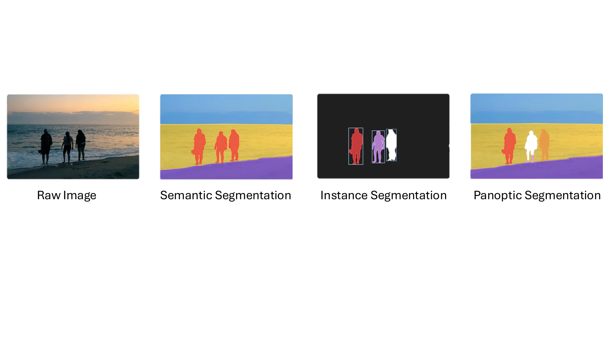
Segmentation partitions an image, a video, or a 3D scan into meaningful regions. Before deep learning it was a mid-level grouping problem, clustering pixels by similarity somewhere between low-level edge detection and high-level recognition; learned models turned it into dense prediction, with class labels, instance identities, and temporal consistency attached to every region. Figure 6.2 shows the principal segmentation map types produced on a common scene.
6.1.2.1Task Definition#
Semantic Segmentation: Given an input image , semantic segmentation assigns a class label to every pixel, producing a dense label map
| (6.4) |
where is the number of classes; instances of the same class are not distinguished.
Instance and Panoptic Segmentation: Instance segmentation detects and segments each object instance separately. The output is a set of labeled masks
| (6.5) |
where is the binary mask of the -th instance and its class; masks may overlap, and only countable thing classes are covered. Panoptic segmentation keeps the same output form but requires the masks to form a non-overlapping partition of the image that covers thing instances and stuff regions alike, each stuff class as a single mask.
Video Segmentation: Given a video clip , video segmentation predicts temporally consistent masks across frames, output as a set of mask tubes
| (6.6) |
each tracking an object or region over time, with semantic, instance, and panoptic variants as above.
3D Segmentation: Given a point cloud with and optional color or intensity, 3D semantic segmentation labels every point,
| (6.7) |
and 3D instance and panoptic segmentation predict point masks under the same set form and overlap constraints as their image counterparts; voxels or mesh vertices take the place of points for other 3D representations. The definitions carry over unchanged. What changes is the input: the points are unordered, unevenly spaced, and sparse, and that is where 3D methods depart from image methods.
6.1.2.2Methodology#
Figure 6.3 summarizes the method families surveyed below.
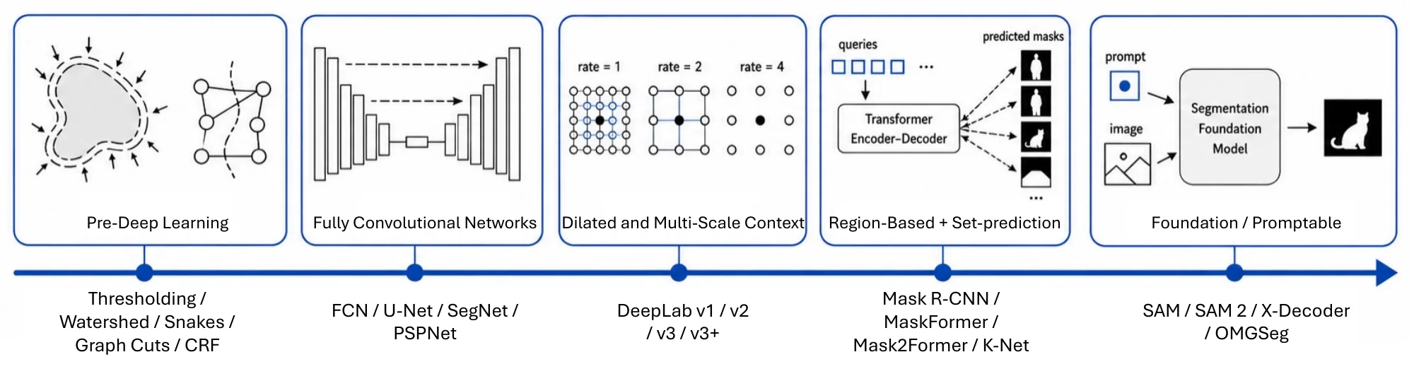
Before Deep Learning. Classical segmentation grouped pixels either by appearance or by minimizing an energy. The first family includes thresholding of pixel intensities [450], region growing that merges similar neighbors [451], -means clustering in feature space [452], and the watershed transform, which treats the image as a topographic surface and segments by catchment basins [453]. The second family includes active contours (snakes) that evolve a curve toward object boundaries [454], graph cuts that solve certain segmentation energies to global optimality [455], and Markov and conditional random fields that impose spatial coherence probabilistically [456, 457]; the last of these carried over directly into early learning-based segmenters.
Fully Convolutional Networks. FCNs [127] replace fully connected layers with convolutions, enabling end-to-end dense prediction at arbitrary input size. U-Net [174] adds a symmetric encoder–decoder with skip connections that fuse low- and high-level features, SegNet [458] reuses max-pooling indices for cheap upsampling and boundary recovery, and PSPNet [459] aggregates global and local context through pyramid pooling.
Dilated and Multi-Scale Context Modeling (DeepLab Series). The DeepLab series introduces atrous (dilated) convolution to enlarge the receptive field without losing resolution (v1 [460]), Atrous Spatial Pyramid Pooling for multi-scale context (v2 [461], refined with batch normalization and stronger backbones in v3 [462]), and an encoder–decoder that recovers boundary detail from low-level features (v3+ [463]).
Region-Based Mask Prediction (Mask R-CNN Family). Mask R-CNN [131] extends Faster R-CNN with a parallel mask branch and ROIAlign, which removes the quantization error of ROI pooling and makes pixel-accurate masks possible. PANet [464], Hybrid Task Cascade [465], and PointRend [466] refine it through better feature flow, cascaded box–mask prediction, and point-wise boundary rendering respectively; this two-stage, region-based family dominated instance segmentation until transformers arrived.
Transformer Backbones and Representation Learning. Transformer-based segmentation, following DETR, favors unified query-based formulations that bridge detection and segmentation, predict masks end-to-end without hand-crafted post-processing, and allow joint learning across tasks and modalities. The first step was the backbone: SETR [467] applies a pure ViT to semantic segmentation with a simple decoder, SegFormer [468] pairs a lightweight hierarchical transformer with an MLP decoder for a favorable accuracy–efficiency trade-off, and Swin Transformer [469] uses shifted-window attention to produce CNN-like multi-scale features and has become a default segmentation backbone. Self-supervised pretraining such as MAE [470] supplies ViT backbones that transfer well to dense prediction.
Query-based Transformer Segmentation. Query-based methods cast segmentation as set prediction with object or mask queries. MaX-DeepLab [471] is the first purely mask-based panoptic framework without box supervision; MaskFormer [472] unifies semantic, instance, and panoptic segmentation by predicting mask embeddings with class labels; K-Net [473] treats segmentation as kernel prediction with iterative refinement; and Mask2Former [474] adds masked cross-attention and multi-scale decoding, setting a strong baseline across all three tasks. QueryInst [475] and Panoptic SegFormer [476] are variants that respectively generate instance-specific kernels from queries and decouple semantic from instance queries.
Video and Multimodal Transformer-based Segmentation. VisTR [477] predicts spatio-temporal mask tubes end-to-end from object queries; Video K-Net [478] unifies video semantic, instance, and panoptic segmentation by associating queries across time; and TubeFormer [479] adds tube-level attention for long-term consistency. X-Decoder [480] and OMGSeg [481] use multimodal pretraining to cover open-vocabulary, class-agnostic, image and video segmentation within a single model.
SAM series. SAM [138] made segmentation promptable: trained on the SA-1B dataset of over one billion masks, it decouples a heavy image encoder from a light prompt-conditioned mask decoder and produces masks from points, boxes, or text with strong zero-shot generalization. SAM 2 [482] extends this to video, propagating masks across frames with a memory mechanism while keeping interactive control.
3D Point Cloud Segmentation. Point-cloud segmenters split by how they impose structure on the points (Section 4.2.3). Point-based networks consume raw points: PointNet [132] applies a shared MLP to every point and pools symmetrically, PointNet++ [270] adds hierarchical neighborhoods, DGCNN [483] builds -nearest-neighbor graphs that are recomputed in feature space at every layer, KPConv [484] defines convolution kernels by points placed in space, and RandLA-Net [485] relies on random sampling to scale to scenes of millions of points. Sparse voxel networks such as MinkowskiNet [486] and SPVNAS [176] quantize the points and convolve only occupied voxels, which keeps 3D convolution affordable on room- and street-scale scans. Projection methods take the opposite route: RangeNet++ [487] unrolls a LiDAR sweep into a range image, runs a 2D segmenter in real time, and projects the labels back onto the points. Transformers entered with Point Transformer [282], and Point Transformer V3 [488] replaces exact neighbor search with serialized point orderings so that attention scales to large scenes.
Instance segmentation in 3D retraces the 2D history. PointGroup [489] predicts per-point offsets toward instance centers and clusters the shifted points, a bottom-up grouping; Mask3D [490] applies Mask2Former-style queries to sparse voxel features and predicts instance masks directly. Because 3D labels remain scarce, open-vocabulary 3D segmentation mostly borrows from 2D foundation models: OpenScene [39] distills CLIP-aligned pixel features into points, and OpenMask3D [491] classifies class-agnostic 3D instance masks with CLIP features aggregated over multi-view images.
| Dataset | Purpose | Classes | Resolution | Samples | ||
| Train | Valid | Test | ||||
| 2D | ||||||
| Pascal VOC [444] | Generic | 21 | Variable | 1464 | 1449 | Private |
| MS COCO [440] | Generic | 80+ | Variable | 82,783 | 40,504 | 81,434 |
| ADE20K [492] | Generic | 150 | Variable | 20,210 | 2,000 | 3,000 |
| COCO-stuff [493] | Generic | 172 | Variable | 118,000 | 5,000 | 20,000 |
| IDD [494] | Urban/Driving | 34 | Variable | 6,993 | 981 | 2,029 |
| Dark Zurich [495] | Urban/Driving | 19 | 19201080 | 8,377 | 50 | 151 |
| ACDC [496] | Driving | 30 (19) | 2048 1024 | 1,600 | 406 | 2,000 |
| PartImageNet [497] | Generic-Part | 158 | Variable | 16,540 | 2,957 | 4,598 |
| SiftFlow [498] | Outdoor | 33 | 256256 | 2,688 | - | - |
| BSD [499] | Generic | 30 | Variable | 12,000 | - | - |
| Youtube-Objects [500] | Generic/Video | 10 | 480360 | 126 | - | - |
| Cityscapes [501] | Urban | 30 (8) | 2048 1024 | 2975 | 500 | 1525 |
| CamVid [502] | Urban/Driving | 32 | 960720 | 701 | - | - |
| Mapillary Vistas [503] | Street | 65 | - | 18,000 | - | - |
| 3D | ||||||
| NYU-D V2 [504] | Indoor | 40 (13) | 640480 | 795 | - | 654 |
| SUN-3D [505] | SfM/Video | - | 640480 | 415 seqs | - | - |
| SUN RGB-D [447] | Indoor | 37 | Variable | 5,285 | - | 5,050 |
| ScanNet [448] | Indoor | 20 | Variable | 1,201 | 312 | 100 |
| SemanticKITTI [506] | LiDAR/Driving | 28 | Point cloud | 19,130 | 4,071 | 20,351 |
6.1.2.3Datasets and Metrics#
Table 6.3 summarizes the main benchmarks. PASCAL VOC [444] anchored the classical semantic-segmentation era with 20 foreground classes and no instance labels. MS COCO [440], with semantic, instance, box, and panoptic annotations over complex object-centric scenes, is the shared testbed for all three modern task types. Cityscapes [501] and Mapillary Vistas [503] specialize to street scenes, the latter stressing long-tail classes and diverse geographies, and ADE20K [492] targets holistic scene parsing over 150 object and stuff classes. The 3D rows of the table cover indoor RGB-D scans (NYU-D V2, SUN RGB-D, ScanNet) and outdoor LiDAR (SemanticKITTI), and S3DIS [507] is a further indoor standard.
Segmentation evaluation reuses IoU (Section 6.1.1) with masks in place of boxes. For semantic segmentation the headline metric is the mean Intersection over Union (mIoU),
| (6.8) |
where is the number of classes and , , count the true-positive, false-positive, and false-negative pixels for class . Because the average is unweighted, mIoU is sensitive to rare classes, which is one motivation behind ADE20K and Mapillary Vistas; pixel accuracy is dominated by frequent classes (e.g., , sky, road) and is less informative.
For instance segmentation, the COCO mask-AP protocol matches predictions to ground truth by mask IoU and averages AP over IoU thresholds –. For panoptic segmentation, Panoptic Quality [243] is , the average IoU of matched segments times the F1 score over matched, false-positive, and false-negative segments, treating things and stuff uniformly. For video object segmentation, the DAVIS metric averages region similarity (, mask IoU) and contour accuracy (, computed on mask boundaries). 3D semantic segmentation reports the same mIoU computed over points or voxels, and 3D instance segmentation on ScanNet reports AP at mask IoU thresholds averaged over –, with AP50 and AP25 as looser slices.
| Method | Backbone | ADE20K mIoU | Cityscapes mIoU | COCO Mask AP | COCO PQ | Year |
| FCN family and dilated convolution | ||||||
| FCN-8s [127] | VGG-16 | 29.4 | 62.7 | – | – | 2015 |
| PSPNet [459] | R101 | 43.3 | 80.2 | – | – | 2017 |
| DeepLab v3+ [463] | Xception-65 | 45.6 | 82.1 | – | – | 2018 |
| Region-based instance segmentation | ||||||
| Mask R-CNN [131] | R50-FPN | – | – | 35.4 | – | 2017 |
| HTC [465] | R50-FPN | – | – | 38.4 | – | 2019 |
| Transformer backbones | ||||||
| SETR-MLA [467] | ViT-L | 50.3 | 82.2 | – | – | 2021 |
| SegFormer-B5 [468] | MiT-B5 | 51.0 | 84.0 | – | – | 2021 |
| Swin-L + UperNet [469] | Swin-L | 53.5 | – | – | – | 2021 |
| Universal query-based segmentation | ||||||
| MaskFormer [472] | Swin-L | 55.6 | – | – | 52.7 | 2021 |
| Mask2Former [474] | Swin-L | 57.7 | – | 50.1 | 57.8 | 2022 |
Table 6.4 reports results across these four protocols. The clearest trend is on semantic segmentation, where ADE20K mIoU has roughly doubled in under a decade, from FCN-8s’s to Mask2Former’s ; the largest single jumps track two shifts, first to transformer backbones (SETR, SegFormer, Swin-L) and then to universal query-based formulations. That second shift is what unifies the table: MaskFormer is the first entry to report semantic mIoU and panoptic PQ within one framework, and Mask2Former extends the same architecture to all three tasks with competitive results on each. Instance segmentation followed a partly separate path, climbing from Mask R-CNN () and HTC () on R50-FPN to once Mask2Former is paired with a Swin-L backbone, which confirms that transformer backbones lift mask quality at the instance level as well, not only semantic accuracy.
6.1.2.4Challenges#
The cost of self-attention at high resolution, over long video, and on dense 3D data sharpens the accuracy–speed tension noted for detection, and two problems are specific to segmentation. Long-video, multi-object consistency is hard. Holding spatial precision and temporal coherence together remains difficult in cluttered scenes, particularly for video panoptic segmentation and segmentation-based multi-object tracking, where objects enter, leave, and occlude one another over long horizons. Segmentation is moving toward the open world. The field is shifting from fixed label sets to class-agnostic, open-vocabulary, and multimodal settings, in which language and other auxiliary signals are folded in to improve spatial reasoning and adaptability, a direction that SAM, X-Decoder, and OMGSeg already anticipate.
6.1.3Keypoint and Landmark Detection#
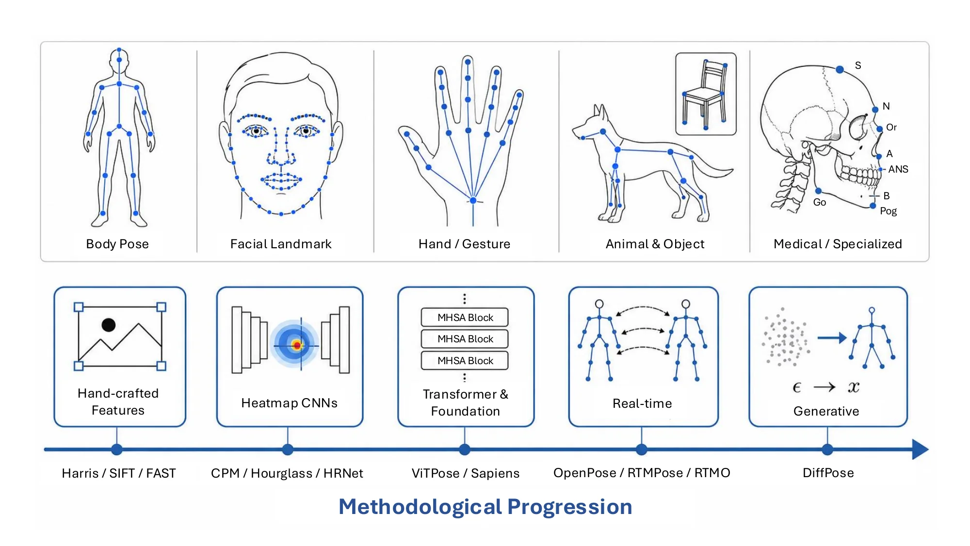
Keypoint and landmark detection localizes a set of semantically consistent, precisely positioned points that characterize object geometry in images or videos: eye corners, skeletal joints, or structurally distinctive parts of man-made objects. Compared with region-based representations, keypoints give a sparser, explicitly geometric encoding that often survives deformation, rotation, and partial occlusion. Figure 6.4 summarizes the task families and the method families surveyed below.
6.1.3.1Task Definition#
Given an input image , a parametric model estimates a set of point locations
| (6.9) |
where each is the image coordinate of a salient visual or structural element. Landmark detection fixes a predefined semantic identity for each point (a particular eye corner, a particular joint); the two terms are otherwise used interchangeably.
3D keypoint detection predicts instead. From images, the depth of each point must be inferred; from depth maps or point clouds , it is observed, and the detector chooses or regresses points on the measured surface. For human pose, 3D joints are usually expressed in camera coordinates relative to a root joint (the pelvis), which leaves global depth unconstrained, as a single image cannot fix it.
The task varies along three axes. The input modality sets what geometry is directly available: most detectors work on 2D images (RGB, grayscale, or infrared), where keypoints must be inferred from appearance alone, whereas point clouds expose spatial structure directly; RGB-D or RGB-infrared fusion adds robustness in clutter and poor lighting, and video supplies temporal continuity through motion blur and transient occlusion. The prediction target ranges from planar image coordinates, which underpin most benchmarks, to 3D keypoints required in robotics and autonomous driving, to 4D trajectories tracked over time. The application scenario fixes what the points mean. Research has concentrated on humans: body joints for pose estimation, facial landmarks for expression recognition and identity verification, and finger joints for gesture-based interaction and sign language recognition [508]. Keypoints are also defined on everyday items, industrial parts, and vehicles for manipulation, inspection, and driving (e.g., , monocular 3D detection from vehicle keypoints [509]), on animals for behavior analysis (multi-animal DeepLabCut [510]), and on anatomical structures in medical imaging, where universal landmark detectors cover several modalities and anatomies [511].
6.1.3.2Methodology#
Classical pipelines combined local feature detectors with statistical shape models that handled occlusion and deformation through explicit geometric constraints. Moravec [512], Harris [257], and Shi–Tomasi [513] corners were followed by SIFT [111], SURF [514], FAST [515], BRIEF [516], and ORB [517], which improved scale invariance, speed, and robustness. For faces and hands, active shape models [518], active appearance models [519], and constrained local models with regularized mean-shift fitting [520] provided the parametric frameworks.
Learning-based detection began with supervised descent for face alignment [521] and, in 2014, with DeepPose [258], which regressed human joints directly with a deep network. Heatmap regression then dominated through 2020: Tompson et al. [522, 523] coupled convolutional networks with graphical models, convolutional pose machines [524] and stacked hourglass networks [256] refined heatmaps over repeated stages, and HRNet [525] kept a high-resolution branch throughout the network for precise localization.
Multi-person estimation splits into two strategies. Top-down methods detect each person first and then estimate keypoints inside the box, which is accurate but scales with the number of people; bottom-up methods predict all keypoints at once and then group them, which is faster but makes grouping the hard part. Part Affinity Fields [526], consolidated as OpenPose [527], are the canonical bottom-up design; YOLO-Pose [528], RTMPose [529], and RTMO [530] push real-time multi-person estimation across both paradigms.
Vision transformers and foundation models made keypoint detection general-purpose: ViTPose [531] set simple transformer baselines for human pose in 2022, and Sapiens [532] in 2024 provides a single foundation model for human-centric vision tasks.
3D human pose estimation grew out of these 2D detectors. Lifting methods take detected 2D keypoints as input and regress the 3D joints: a fully connected network on 2D joints alone was a strong baseline [533], temporal convolutions over 2D pose sequences (VideoPose3D [534]) and spatio-temporal transformers (MotionBERT [535]) use motion to reduce the depth ambiguity, and DiffPose [536] casts lifting as diffusion. Direct methods predict 3D from pixels, as in the volumetric heatmaps of Pavlakos et al. [537]. With a calibrated multi-view rig most of the ambiguity disappears, and learnable triangulation [538] fuses per-view heatmaps into a 3D estimate. Recovering a full body mesh rather than a joint set is taken up with human motion in Section 8.4.
Classical corner detectors were in turn replaced by learned ones: SuperPoint [539] learns detection and description jointly under self-supervised homographic adaptation, DISK [540] selects keypoints with a reinforcement-style objective, and SuperGlue [541] and the detector-free LoFTR [542] recover dense correspondences directly. These serve as correspondence rather than semantic points and are the workhorses of the structure-from-motion, visual-odometry, and SLAM pipelines in the spatial-localization section that follows.
On point clouds, keypoints mostly serve registration and pose estimation. Intrinsic Shape Signatures [543] select points whose local neighborhood has a distinctive eigenvalue structure; USIP [544] learns, without labels, detectors that stay stable under rigid transformation, and D3Feat [545] predicts a detection score and a descriptor for every point, the 3D analogue of SuperPoint. Category-level 3D keypoints are a different kind: Suwajanakorn et al. [546] discover keypoints that are consistent across instances of a category through a relative-pose objective, and kPAM [547] uses such keypoints as the interface for robotic manipulation. Keypoint-based 6D object pose, which predicts the 2D projections of 3D model keypoints and solves PnP, belongs to pose estimation (Section 6.2.5).
Table 6.5 reports COCO Keypoints (val2017) results for the CNN, transformer, and real-time families.
| Method | Backbone | Input | #Params (M) | GFLOPs | AP | AP50 | AP75 | AR | Year |
| HRNet-W32 [525] | HRNet-W32 | 256192 | 28.5 | 7.1 | 74.4 | 90.5 | 81.9 | 79.8 | 2020 |
| HRNet-W48 [525] | HRNet-W48 | 384288 | 63.6 | 32.9 | 76.3 | 90.8 | 82.9 | 81.2 | 2020 |
| YOLOv5s6-Pose [528] | YOLOv5-s | 960960 | 15.1 | – | 63.8 | 87.6 | 69.6 | 70.4 | 2022 |
| YOLOv5m6-Pose [528] | YOLOv5-m | 960960 | 41.4 | – | 67.4 | 89.1 | 73.7 | 73.9 | 2022 |
| YOLOv5l6-Pose [528] | YOLOv5-l | 960960 | 87.0 | – | 69.4 | 90.2 | 76.1 | 75.9 | 2022 |
| ViTPose-B [531] | ViT-B | 256192 | 86 | – | 75.8 | – | – | 81.1 | 2022 |
| ViTPose-L [531] | ViT-L | 256192 | 307 | – | 78.3 | – | – | 83.5 | 2022 |
| ViTPose-H [531] | ViT-H | 256192 | 632 | – | 79.1 | – | – | 84.1 | 2022 |
| RTMPose-s [529] | CSPNeXt-s | 256192 | 5.5 | 0.68 | 69.6 | – | – | – | 2023 |
| RTMPose-m [529] | CSPNeXt-m | 256192 | 13.6 | 1.93 | 73.6 | – | – | – | 2023 |
| RTMPose-l [529] | CSPNeXt-l | 256192 | 27.7 | 4.16 | 74.8 | – | – | – | 2023 |
| RTMO-s [530] | CSPDarkNet | 640640 | 9.9 | – | 67.7 | 87.8 | 73.7 | 71.5 | 2024 |
| RTMO-m [530] | CSPDarkNet | 640640 | 22.6 | – | 70.9 | 89.0 | 77.8 | 74.7 | 2024 |
| RTMO-l [530] | CSPDarkNet | 640640 | 44.8 | – | 72.4 | 89.9 | 78.8 | 76.2 | 2024 |
6.1.3.3Datasets and Metrics#
Keypoint datasets are mostly embedded in broader pose and action benchmarks rather than built in isolation; Table 6.6 lists the most used. Human body datasets are the most mature and trace the field’s expansion: MPII [548] and COCO Keypoints [440] fixed in-the-wild 2D evaluation, PoseTrack [549] added temporal association in video, Human3.6M [550] supplies controlled multi-view 3D ground truth for 2D-to-3D lifting, DensePose [551] replaces sparse joints with dense surface correspondences, and CrowdPose [552] stresses crowded, occluded scenes. Face datasets moved from large pose variation (AFLW [553]) and high-density annotation (HELEN [554]) to occlusion (COFW [555]), the standardized 68-point protocol of 300-W [556] and its large-pose synthetic extension 300-W-LP [557], and the 98-point, hard-condition WFLW [558]. Hand datasets contend with fine articulation and self-occlusion through multi-view capture (CMU Panoptic HandDB [559]), synthetic 3D labels (RHD [560]), real 3D pose and shape (FreiHAND [561]), and interacting hands (InterHand2.6M [562]). Animal-Pose [563] and AP-10K [564] carry the human recipe to animals across species, while ApolloCar3D [565] and KeypointNet [566] define keypoints on rigid vehicles and 3D object categories.
| Dataset | Year | Domain | Mod. | KP | #Samples (train / val / test) |
| Human body | |||||
| MPII [548] | 2014 | In-the-wild body | 2D | 16 | 25K images (train+test) |
| COCO Keypoints [440] | 2014 | In-the-wild multi-person | 2D | 17 | 57K / 5K / 20K images |
| PoseTrack [549] | 2017 | Video body tracking | 2D | 15 | 593 / 170 / 375 videos |
| Human3.6M [550] | 2014 | Indoor multi-view body | 3D | 32 | 3.6M frames, 11 subjects |
| DensePose [551] | 2018 | Dense body surface | 2D | SMPL surface | 50K images (COCO subset) |
| CrowdPose [552] | 2019 | Crowded multi-person | 2D | 14 | 10K / 2K / 8K images |
| Face | |||||
| AFLW [553] | 2011 | In-the-wild face | 2D | 21 | 25K faces (22K images) |
| HELEN [554] | 2012 | High-resolution face | 2D | 194 | 2K / – / 330 images |
| COFW [555] | 2013 | Occluded face | 2D | 29 | 1.3K / – / 507 images |
| 300-W [556] | 2013 | Aggregated face | 2D | 68 | 3.1K / – / 689 images |
| 300-W-LP [557] | 2016 | Large-pose synthetic face | 2D | 68 | 61K images |
| WFLW [558] | 2018 | In-the-wild face (challenging) | 2D | 98 | 7.5K / – / 2.5K images |
| Hand | |||||
| CMU Panoptic HandDB [559] | 2017 | Multi-view hand | Multi-view | 21 | 14K manual + bootstrapped |
| RHD [560] | 2017 | Synthetic hand | 2D + 3D | 21 | 41K / – / 2.7K frames |
| FreiHAND [561] | 2019 | Real hand pose + shape | 3D | 21 | 33K / – / 4K samples |
| InterHand2.6M [562] | 2020 | Two-hand interaction | 3D | 42 | 2.6M frames |
| Animal & Object | |||||
| Animal-Pose [563] | 2019 | 5-class mammal pose | 2D | 20 | 4K images |
| AP-10K [564] | 2021 | 54-species animal pose | 2D | 17 | 10K images |
| ApolloCar3D [565] | 2019 | Vehicle keypoints (driving) | 2D | 66 | 5.3K images |
| KeypointNet [566] | 2020 | Multi-category 3D objects | 3D | 5–23 | 8.3K models |
Metrics measure the distance between predicted and ground-truth points, normalized for scale. The End-Point Error (EPE) is the raw Euclidean distance. The Normalized Mean Error (NME) divides it by a reference length:
| (6.10) |
where and denote the predicted and ground-truth locations of the -th keypoint, and is a task-dependent normalization factor (e.g., , inter-ocular distance for faces). The Percentage of Correct Keypoints (PCK) instead thresholds the error,
| (6.11) |
where controls the tolerance and is the reference scale, giving an accuracy rate that is easy to compare across methods; the Cumulative Error Distribution (CED) curve and its Area Under the Curve (AUC) summarize behavior across thresholds.
For large-scale benchmarks, Object Keypoint Similarity (OKS) incorporates object scale and keypoint-specific uncertainty,
| (6.12) |
Here denotes the object scale (the square root of the segmented area), is a per-keypoint normalization constant calibrating the fall-off, and is the ground-truth visibility flag for keypoint , where indicates unlabeled, indicates labeled but occluded, and indicates labeled and visible. OKS plays the role of IoU in computing average precision and recall on MS COCO [440]. For 3D human pose, the Mean Per-Joint Position Error (MPJPE) averages the Euclidean joint error in millimeters after aligning the root joints; PA-MPJPE applies a Procrustes alignment of scale, rotation, and translation first, and 3DPCK thresholds the error at mm, as on MPI-INF-3DHP [567]. Point-cloud keypoint detectors are scored by repeatability under rigid transformation and, downstream, by registration recall on benchmarks such as 3DMatch [568].
6.1.3.4Challenges#
Robustness in unconstrained scenes is still the first problem [569, 570]: occlusion, extreme pose, and non-rigid deformation leave partial or ambiguous configurations, and symmetric parts (left versus right limbs, the fingers of a self-occluded hand) are routinely swapped. Generalization is the second [571, 572, 573]: keypoint definitions differ across datasets even for the same object class, so models trained on one benchmark transfer poorly to another, and the gap widens for animals, objects, and anatomical structures, where annotation is scarce and demographic or species bias enters the training data. The accuracy–speed tension discussed for detection applies here as well [574, 575]: high-precision models are too heavy for embedded targets, and lightweight ones lose accuracy precisely under occlusion and fast motion.
6.1.4Scene Classification#
Going beyond objects, regions, and keypoints, scene classification (SC) assigns a single semantic label to a whole image describing the environment it portrays [576]. Where object recognition names the things in a picture (“car”, “tree”, “person”), scene classification names the where: “a busy street”, “a serene beach”, “a modern kitchen”. It asks “What kind of place is this?”, a judgment that rests on the global layout and gist of the image rather than on any single object [577, 578], and it supplies the holistic prior on which an embodied or virtual agent conditions its later behavior [579, 580, 219, 581].
6.1.4.1Task Definition#
Formally, scene classification learns a mapping from an image to a label in a predefined category set , or, in the multi-label case, to a subset covering several facets of the scene [582] (“urban” for area, “parking lot” for place, “night” for condition). Beyond the single-/multi-label split, the task is instantiated by domain, with indoor [583] and outdoor [584] scenes, remote-sensing imagery [585, 586], and driving contexts such as highways and tunnels [580], and by modality, extending from still images to video [587] and acoustic scenes [588].
6.1.4.2Methodology#
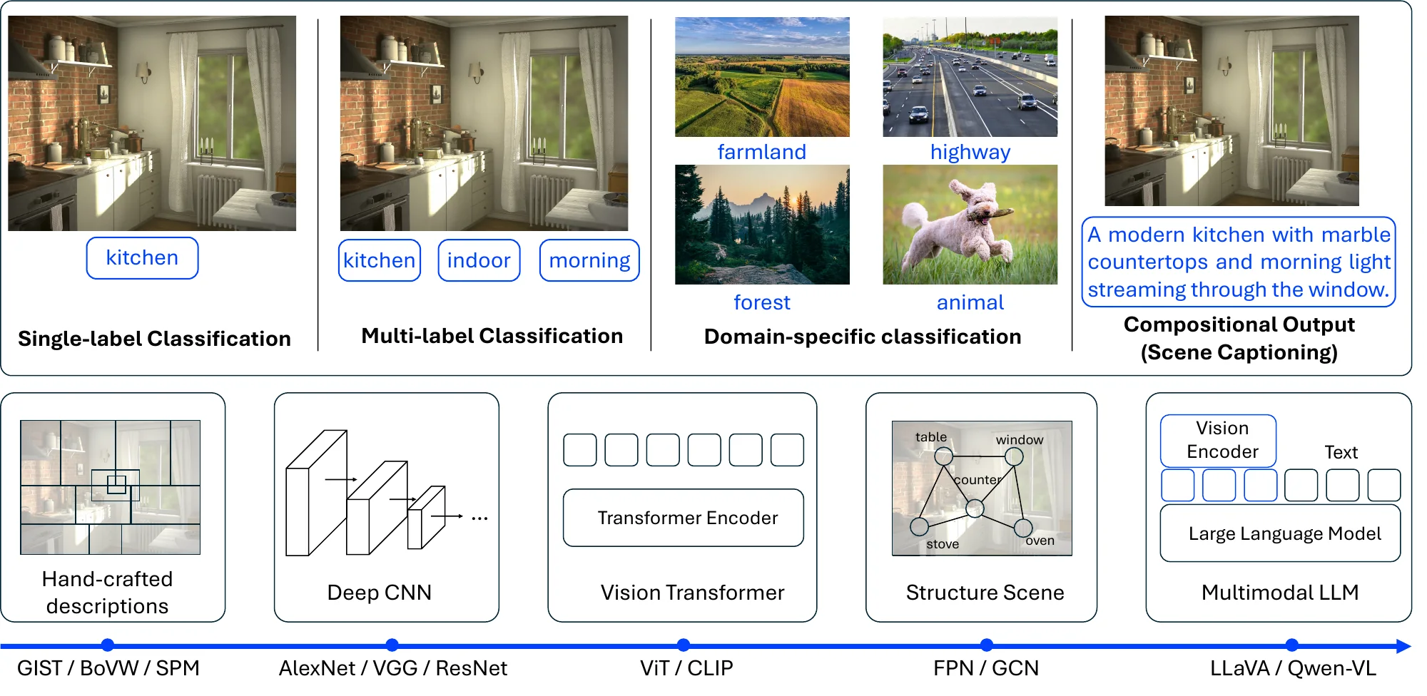
Figure 6.5 summarizes the progression from hand-crafted global descriptors through deep features to vision–language models.
Early methods summarized the whole image into one discriminative vector of low-level texture, color, and gradient statistics. The Spatial Envelope model [589] describes a scene by a few perceptual dimensions (naturalness, openness, roughness, expansion, ruggedness), a descriptor commonly called GIST. Bag-of-Visual-Words (BoVW) [590] treats the image as a histogram of quantized local features such as SIFT [111], discarding most spatial information [591]; Spatial Pyramid Matching (SPM) [592] restores coarse layout by computing BoVW histograms over a pyramid of sub-regions and concatenating them.
Deep networks learn scene features end to end. CNNs [125, 593] such as AlexNet [125], VGG [594], ResNet [23], and DenseNet [595], pre-trained on ImageNet [439, 125], proved to be strong global feature extractors for scenes, and Places-CNN [596] re-trained them on the large-scale Places benchmark to establish the standard transfer recipe. Vision Transformers [142] match or exceed CNNs with a class-token embedding that attends over all patches, in the manner of BERT [42].
A separate line models layout explicitly, since a stadium is recognized by its global oval while a classroom differs from an office by the mid-scale arrangement of desks and blackboard. Multi-scale pooling over the CNN feature hierarchy (FPN-style [597]) captures structure at several scales, and scene graphs [598] make objects and their relations explicit, so that propagating over them with graph convolutional networks [599] yields layout-aware scene features [600].
Vision–language models (VLMs) turn scene classification into open-vocabulary, zero-shot matching. Contrastive models such as CLIP [143] embed the image and the textual names of all candidate classes in one space and pick the most similar class [601], needing no fine-tuning beyond prompt design [602]; the recipe extends to 3D point clouds [368]. Autoregressive multimodal large language models (MLLMs; LLaVA [145], Qwen-VL [603], Gemma 3 [604]) instead generate the label as text in response to an instruction [605]. With rich semantics available for free, the research focus has shifted from one global label toward compositional understanding of what is inside the scene [606].
6.1.4.3Datasets and Metrics#
Table 6.7 lists the standard benchmarks. The small early sets, Scene 15 [592] and the indoor MIT 67 [583], were superseded by SUN 397 [607, 608], which fixed a near-exhaustive category list, and by Places [596, 609], which scaled the same categories to millions of images across its Places205, Places88, Places365-Standard, and Places365-Challenge subsets. NYU Depth v2 [504] and SUN RGB-D [447] add aligned depth and a scene category per image for indoor RGB-D classification.
| Dataset | Year | Domain | Mod. | #Classes | #Images (protocol) |
| Scene 15 [592] | 2006 | Indoor + outdoor, grayscale | 2D | 15 | 4,448 |
| MIT Indoor 67 [583] | 2009 | Indoor | 2D | 67 | 15,620 (80 / 20 per class) |
| SUN 397 [607, 608] | 2010 | Indoor + outdoor | 2D | 397 | 108,754 (50 test per class) |
| Places205 [596] | 2014 | Indoor + outdoor | 2D | 205 | 2.5M |
| Places365-Standard [609] | 2017 | Indoor + outdoor | 2D | 365 | 1.8M |
| Places365-Challenge [609] | 2017 | Indoor + outdoor | 2D | 365 | 8M |
| NYU Depth v2 [504] | 2012 | Indoor | RGB-D | – | 1,449 labeled pairs |
| SUN RGB-D [447] | 2015 | Indoor | RGB-D | – | 10,335 |
Scene classification is evaluated primarily with top-1 accuracy (the fraction of images for which the highest-scoring predicted class matches the ground truth) and top-5 accuracy (the fraction of images where the ground-truth class is among the top five predictions), with the latter especially useful on long-tail benchmarks such as Places-365 and SUN 397. For multi-label settings, the mean Average Precision (mAP) and class-wise F1 are reported instead, mirroring the protocol used in multi-label image recognition.
| Method | Backbone | Places-365 Top-1 | SUN 397 Top-1 | Year |
| Supervised | ||||
| Places365-AlexNet [609] | AlexNet | 53.2 | – | 2017 |
| Places365-VGG [609] | VGG-16 | 55.2 | – | 2017 |
| Places365-ResNet [609] | R152 | 54.7 | – | 2017 |
| Vision-language zero-shot | ||||
| CLIP [143] | ViT-L/14 | – | 63.2 | 2021 |
Table 6.8 reports results on the two most-cited scene benchmarks. Supervised CNNs on Places-365 cluster in a narrow band of roughly – top-1, with diminishing returns from AlexNet to ResNet, while CLIP reaches top-1 on SUN 397 zero-shot [143], on par with supervised scene classifiers without any target-set training.
6.1.4.4Challenges#
Closed-set accuracy on Places-365, SUN 397, and MIT 67 is now recovered zero-shot by CLIP [143] and by MLLMs (LLaVA [145], Qwen-VL [603], Gemma 3 [604]), so “what kind of place is this” is no longer the frontier. The task has climbed a granularity ladder, from one label to attribute sets to grounded, compositional description across image, video, and 3D, and the open problems sit at that richer end, where MLLMs are weaker than their coarse-label accuracy suggests.
Fine-grained and long-tail discrimination. MLLMs still trail dedicated classifiers and CLIP-style models on fine-grained and long-tail categories, where the distinction between, e.g., , a “bistro” and a “brasserie” turns on subtle cues [610].
Compositional and spatial grounding. The natural output is no longer a label but a description whose claims can be grounded in specific objects and layouts [606]. MLLMs describe fluently but ground weakly: objects are referenced vaguely rather than by region or box, and the persistent failure is structural rather than semantic, since models name the constituents of a scene correctly yet err on relative layout, depth ordering, orientation, and cross-view or 3D consistency. The cause is representational: 2D patch tokens are optimized for semantic alignment with language, not geometry, so fine spatial cues are lost once flattened into the language stream, and spatial-cognition benchmarks show even strong MLLMs degrading sharply as tasks move from naming toward layout and 3D reasoning [611, 612].
Hallucination and faithfulness. Free-form description reintroduces a failure mode that closed-set classification never had: MLLMs assert objects, attributes, or relations absent from the image, and their reasoning traces rarely point to verifiable spatial evidence [612].