The 2D representations are the most direct and information-dense entry point into spatial intelligence: images and videos provide a regular, discretely sampled grid over the visual field, on top of which a family of structured maps can be defined to expose geometric and semantic properties of the underlying scene. We organize this section around seven such representations (Figure 4.1): the raw image/video tensor itself, and six derived maps: segmentation, depth, surface normal, edge, optical flow, and 2D keypoint representations. All seven share the image grid as their domain, which makes them straightforward to fuse with one another and to consume with convolutional or transformer backbones; what differs is what each representation exposes: appearance, semantics, geometry, boundaries, motion, or sparse structure.
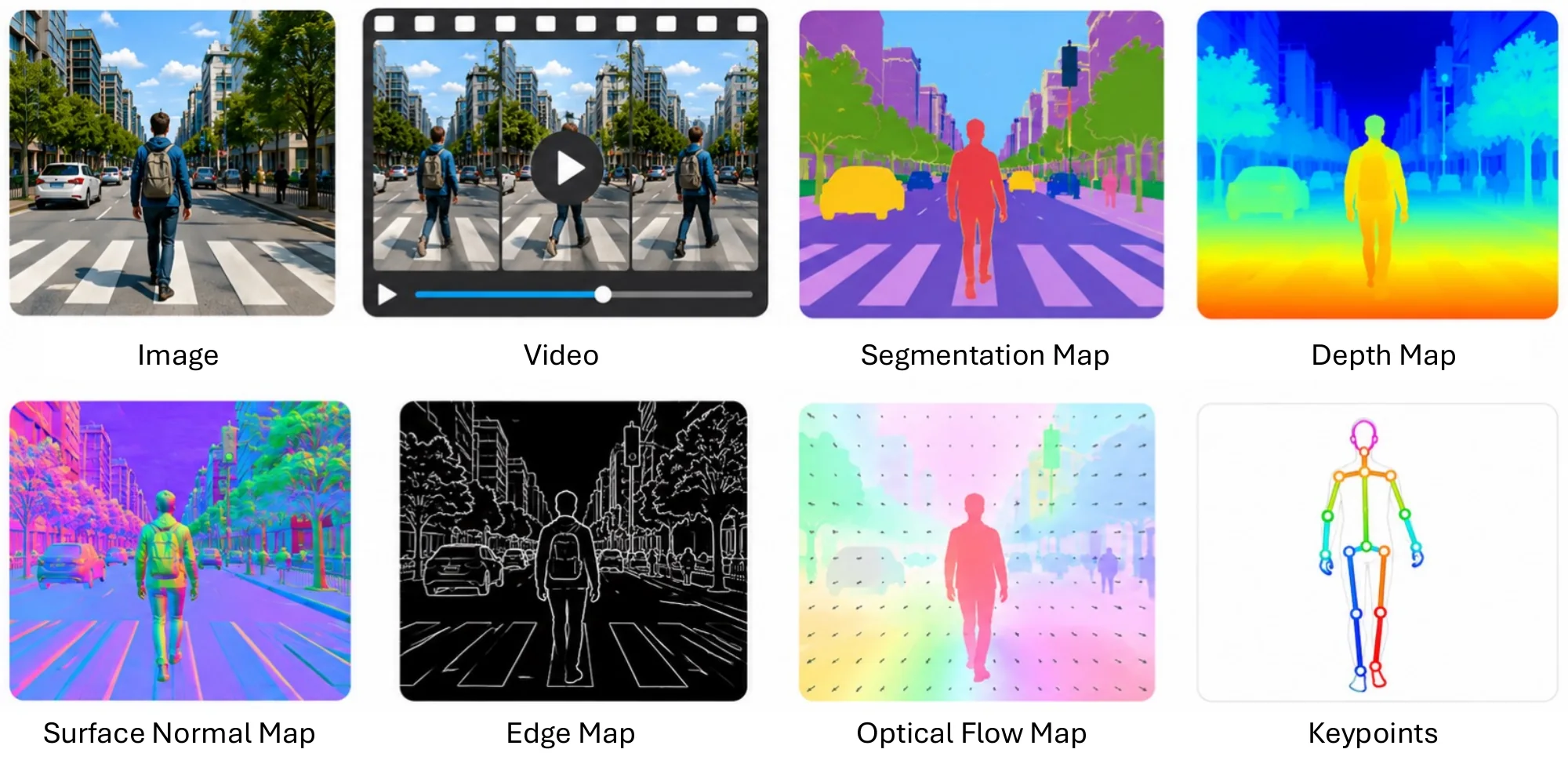
4.1.1Image and Video Representations#
An image can be modeled as a discrete sampling of a continuous visual signal over a 2D spatial domain. Formally, a digital image is represented as a function
| (4.1) |
where denotes the image grid, is the number of channels (e.g., , for grayscale, for RGB), and each pixel value encodes intensity or color information at a discrete spatial location [233, 234]. In practice, images are stored as finite tensors , where and denote image height and width.
A video extends this representation by introducing a temporal dimension. Given a sequence of frames sampled over time, a video can be written as
| (4.2) |
or equivalently as a 4D tensor , where denotes the number of frames [234]. This formulation preserves spatial structure within each frame while enabling the modeling of temporal dynamics across frames. From a computational perspective, images and videos are treated as structured arrays of numerical values that can be efficiently processed using linear algebra operations and convolutional kernels. This regular grid structure enables weight sharing, local receptive fields, and efficient parallel computation, forming the basis of CNNs and their spatiotemporal extensions [235, 236]. In modern deep learning systems, image and video tensors may undergo normalization, resizing, patch embedding, or tokenization before being fed into neural architectures, including CNNs and vision transformers [142, 237]. For video inputs, spatiotemporal extensions either inflate 2D kernels into 3D convolutions [238, 239] or extend self-attention across space and time, as in the family of video transformers [240, 241].
4.1.2Segmentation Maps#
A segmentation map is a semantic representation that assigns a label or a mask to each pixel, thereby partitioning visual data into meaningful regions such as objects, object parts, or background categories [234, 242]. For a single image defined on , segmentation can be written as a mapping
| (4.3) |
where is a set of labels. In semantic segmentation (SS), denotes the class label of pixel . In instance segmentation (IS), the output is a set of masks with associated class labels , where each corresponds to an object instance [127, 131]. Panoptic segmentation (PS) unifies SS and IS by predicting a single, non-overlapping labeling of pixels that distinguishes both “stuff” and countable object instances [243].
These tasks extend naturally to videos. Given a sequence of frames , video semantic segmentation (VSS) predicts per-frame semantic labels , while video instance segmentation (VIS) predicts instance masks with temporal consistency across frames, often requiring instance association (tracking) over time [242]. Video panoptic segmentation (VPS) further combines VSS and VIS, producing temporally consistent panoptic outputs and is commonly evaluated with metrics that account for both segmentation quality and tracking consistency [242]. Closely related settings include video object segmentation (VOS) [244], which segments foreground objects across time under semi-supervised or unsupervised protocols, and referring segmentation, which predicts masks grounded by natural language expressions in images (RIS) [245] or videos (RVOS) [246]. Segmentation maps are typically formed by dense prediction models that produce either hard labels or per-pixel class probabilities (and, for instance-level tasks, a set of object masks and scores). A key advantage of segmentation is its explicit and interpretable structure: it converts low-level pixels into object- and region-level representations that support downstream reasoning and decision-making, and it can be fused naturally with geometry (e.g., , depth, normals) and language in multimodal systems [242]. Consequently, segmentation maps are central to applications such as autonomous driving, medical image analysis, robotic manipulation, visual editing, and human-computer interaction.
4.1.3Depth Maps#
A depth map is a geometric representation that augments a 2D image with per-pixel distance information, describing the spatial layout of a scene from a given viewpoint [234]. Formally, given an image domain , a depth map is a scalar function
| (4.4) |
where denotes the distance from the camera center to the first visible surface along the viewing ray corresponding to pixel . Depending on the sensing modality and formulation, this value may represent metric depth, inverse depth, or disparity [112]. Depth maps can be obtained through multiple mechanisms, including stereo vision via triangulation [112], active sensors such as structured-light or time-of-flight cameras [247], and learning-based monocular depth estimation [55]. When combined with known camera intrinsics, a depth map enables the back-projection of image pixels into 3D space, thereby serving as a bridge between 2D image representations and 3D geometry. A key advantage of depth maps lies in their compact, image-aligned structure, which allows them to be processed using standard convolutional architectures and easily fused with the RGB appearance information. Compared to volumetric representations, depth maps are memory-efficient while still encoding meaningful geometric cues. As a result, they are widely used in applications such as 3D reconstruction, novel view synthesis [119], robotic navigation, and autonomous driving [173].
4.1.4Surface Normal Maps#
A surface normal map is a geometric representation that encodes local surface orientation at each pixel of an image. Given an image domain , a surface normal map assigns to each pixel a unit vector
| (4.5) |
where represents the direction of the surface normal in camera or world coordinates, and denotes the unit sphere. Surface normal maps can be derived from depth maps or 3D geometry via local differentiation, or directly estimated from RGB images using learning-based methods [248]. Classical approaches to normal estimation rely on photometric stereo or geometric reconstruction [249], while modern methods employ CNNs to regress surface normals from monocular images [250]. Regardless of the estimation procedure, surface normal maps remain image-aligned and encode rich local geometric information that complements depth and segmentation cues. Surface normal maps can capture fine-grained shape and orientation details that may be ambiguous or noisy in raw depth estimates. Because surface normals are invariant to absolute depth scale, they provide robust geometric constraints for scene understanding. Consequently, surface normal maps are widely used in applications such as 3D reconstruction, object pose estimation, scene layout analysis, realistic rendering, and as auxiliary supervision in multi-task learning [250].
4.1.5Edge Maps#
An edge map is a structural representation that highlights salient intensity or color discontinuities in an image, which often correspond to object boundaries and significant geometric transitions [251]. Given an image , an edge map is typically constructed by measuring local image gradients, for example,
| (4.6) |
where denotes the spatial gradient operator. Classical edge detection methods rely on hand-crafted operators such as Sobel, Laplacian of Gaussian, and the Canny detector [251], while modern learning-based approaches directly predict the edge probabilities using convolutional neural networks [252]. Edge maps may be binary, indicating the presence or absence of an edge, or real-valued, encoding edge strength, orientation, or confidence. The primary advantage of edge maps is their ability to significantly reduce visual complexity while preserving essential geometric structure. This abstraction makes them relatively robust to changes in illumination and appearance. Consequently, edge maps are widely used in image segmentation, contour detection, shape analysis, line drawing, and as intermediate cues for higher-level tasks such as object recognition and depth estimation [234].
4.1.6Optical Flow Maps#
An optical flow map is a motion representation that encodes the apparent 2D displacement of pixels between consecutive frames in a video sequence [253]. Given two image frames and , the optical flow is defined as a vector field
| (4.7) |
where describes the horizontal and vertical displacement of pixel from time to . Classical optical flow estimation relies on assumptions such as brightness constancy and spatial smoothness, leading to variational formulations [253, 254]. More recently, deep neural networks have been proposed to directly regress dense flow fields from image pairs or short video clips [128, 255]. Regardless of the estimation method, the resulting optical flow map remains image-aligned, preserving spatial correspondence with the input frames. The main advantage of optical flow maps is their ability to capture rich dynamic information about scene motion, including object motion, camera motion, and motion parallax, while remaining computationally efficient. As a result, optical flow is a core representation in video analysis and robotic perception tasks such as motion segmentation, action recognition, video interpolation, and visual odometry.
4.1.72D Keypoints#
A 2D keypoint set is a sparse image representation that encodes the image-plane locations of a finite set of semantically or geometrically meaningful points, such as corners, joints, or landmarks [234]. Unlike dense maps that assign a value to every pixel, keypoint representations summarize visual content with a small number of salient points, trading pixel-level coverage for compactness and geometric explicitness. Formally, given an image defined on a domain , a keypoint representation is a set of points
| (4.8) |
where each keypoint corresponds to a specific semantic or geometric entity. In learning-based formulations, keypoints are often represented implicitly as confidence or heat maps:
| (4.9) |
with the keypoint location obtained by finding the maximum or expected value of [256]. 2D keypoints can be obtained using classical feature detectors, such as Harris corners, SIFT, and SURF [257, 111], or through modern deep neural networks that directly regress keypoint locations or predict dense heat maps [258, 256]. Depending on the task, keypoints may represent generic interest points, object-specific landmarks, or articulated structures such as the human body joints. The detection task that produces such a set, including its extension to landmark detection and human pose estimation, is discussed in detail in Section 6.1.3 of Chapter 6. A key advantage of 2D keypoint representations is their sparsity and compactness: they significantly reduce the dimensionality of visual data while preserving critical structural information. This makes keypoints computationally efficient, robust to background clutter, and well-suited for geometric reasoning and correspondence matching. Human pose estimation is a specialized and highly structured instance of 2D keypoint detection that focuses on localizing a predefined set of anatomical landmarks of the human body, such as joints and facial keypoints, in images or videos [259]. In the 2D setting, the task aims to estimate the image coordinates of body joints, typically represented as a set of keypoints , where denotes the number of joints in a human skeletal model. These keypoints are not independent: they are constrained by the underlying human body structure, which is often modeled using kinematic trees, graphical models, or learned structural priors.