Rule-based symbolic spatial reasoning covers the methods that operate over explicit, model-based representations of space (geometric primitives, physical laws, graph connectivity, formal constraints, action rules, or causal mechanisms) rather than over learned latent representations alone. What sets this family apart is that reasoning happens inside a model that can be inspected: its state and transitions are legible, so claims about feasibility, optimality, or safety can be backed by certificates rather than empirical averages, and when a plan fails it fails legibly, as an infeasible inverse kinematics, a violated constraint, a missing precondition, or an inconsistent causal attribution, not as an opaque correlation.
The section surveys six kinds of explicit structure, ordered from the most concrete to the most abstract: geometric and algebraic models of position, orientation, motion, and feasibility; physical models of contact, friction, and stability; topological and graph abstractions of space that turn planning into search; formal constraint systems whose solvers return certified plans or proofs of infeasibility; rule-based and programmatic logic that sequences and supervises actions; and causal models that explain, predict counterfactually, and prescribe interventions.
These paradigms are not isolated alternatives. Modern robotic systems routinely compose them: geometric solvers serve as feasibility oracles inside constraint-based search; behavior trees wrap symbolic plans for fault tolerance; causal action languages compile to SAT; topological maps anchor both classical and learning-based navigation policies. The unifying thread is that each paradigm carries explicit structure (a state, an operator, a constraint, a rule, or a mechanism) that can be inspected, composed, and reasoned about.
7.1.1Geometric and Algebraic Reasoning#
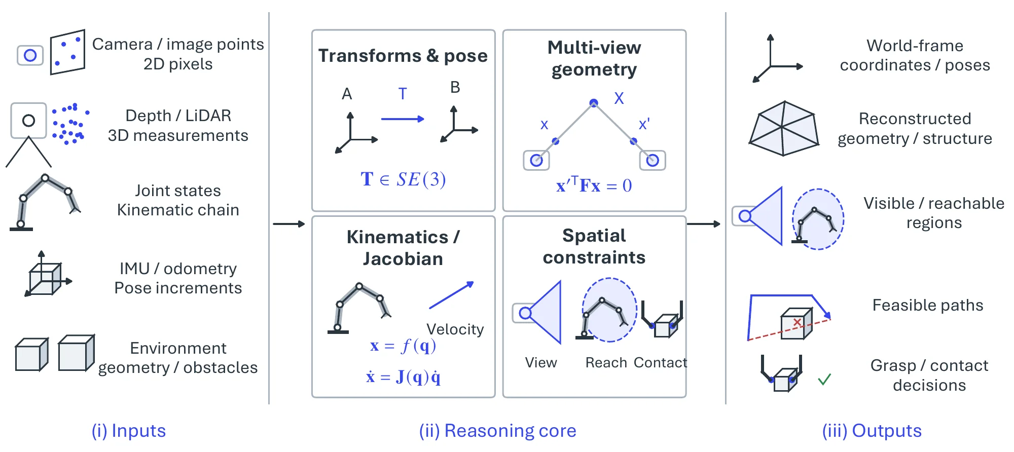
Geometric and algebraic reasoning uses explicit mathematical models of position, orientation, shape, and motion to turn local measurements (image points, depths, joint angles, odometry) into quantities that can be analyzed and verified: where things are in a common frame, what a sensor can see, what a mechanism can reach, and whether a grasp will hold. The same models extend to time-varying settings, where relationships evolve under kinematic and differential constraints and the question becomes not only where entities can be but how they can move. Precision, interpretability, and domain independence have made this the common substrate of robotics [1142, 1143, 1144], AR/VR [112, 1145], and autonomous systems [54, 1146, 165], and the source of the hard constraints that learned components are checked against. Figure 7.1 gives the abstract formulation.
7.1.1.1Task Definition#
Given measurements expressed in local frames (pixels, ranges, joint readings, pose increments) and a system model (sensor calibration, kinematic parameters, environment geometry), geometric reasoning computes a world-frame quantity and a feasibility verdict,
| (7.1) |
where may be a pose, a reconstructed surface, a workspace or visibility region, or a trajectory, and is a predicate that can be checked against the model. In the time-varying case the inputs are indexed over time and becomes a trajectory with reachable sets and feasibility certificates along it.
7.1.1.2Methodology#
Transformation and Pose Representation. Rigid-body relationships between sensors, objects, and mechanisms are elements of the special Euclidean group
| (7.2) |
where is a rotation and a translation; composing them moves measurements across frames. Early robotics parameterized serial chains through the Denavit–Hartenberg convention [1147, 1148], which gives forward kinematics from a minimal set of link parameters. Lie-group formulations instead write motion as exponentials of screw axes, the product-of-exponentials representation [1142, 1143], which is coordinate-free and behaves well where the DH parameterization has discontinuities. Quaternions [1149, 1150] and dual quaternions [1151, 1152] give compact, numerically stable encodings of rotation and screw motion for calibration and sensor fusion.
Projective and Multi-View Geometry. Reasoning from images must recover 3D structure and camera motion from 2D measurements under perspective distortion and scale ambiguity. The constraint between corresponding points in two views is the epipolar condition
| (7.3) |
with the fundamental matrix. The eight-point algorithm [102] solves for linearly, Hartley’s normalization [1153] made it numerically stable, and Nistér’s five-point solver [1154] reaches the minimal case for calibrated cameras. Zhang’s homography-based calibration [692] removed the need for special rigs; the field is consolidated in [112], and structure-from-motion systems such as COLMAP [115] scale it to thousands of images, with RANSAC [101] enforcing the algebraic constraints against outliers throughout.
Jacobian and Differential Formulations. For motion rather than static configuration, the map from configuration to task space,
| (7.4) |
is differentiated to relate velocities,
| (7.5) |
and the Jacobian carries the information about feasibility, singularities, and controllability along a motion. Whitney’s resolved motion rate control [1155] used it to command Cartesian velocities without closed-form inverse kinematics; Nakamura’s damped least squares [1156] trades exactness for stability near singularities; redundancy resolution [1157, 1158] uses null-space motion for secondary objectives; and Khatib’s operational-space formulation [1159] separates task and null-space dynamics so that objectives are written directly in task space.
Visibility and Coverage Geometry. What a sensor at pose can observe is the set
| (7.6) |
with the environment and the obstacles. The Art Gallery theorem [1160, 1161] bounds the number of viewpoints needed for full coverage; polygon visibility [1162] and shortest-path queries [1163] made the computations algorithmic; and Tarabanis et al. [1164] cast sensor planning as geometric optimization over fields of view modeled as cones, frusta, or polygons.
Workspace and Reachability Analysis. The reachable workspace of a mechanism is
| (7.7) |
with the feasible configuration space. Roth [1165] and Gosselin [1166] added performance and dexterity measures so that manipulability is characterized along with reachability; Merlet [1167] classified workspace types; Zlatanov et al. [1168] analyzed constraint-induced singularities; and sampling-based reachability maps [1169] trade closed-form guarantees for empirical coverage in high-dimensional systems.
Contact and Grasp Geometry. Whether a set of contacts can hold an object is decided in wrench space. Ferrari and Canny [1170] model the forces each contact can apply as a convex set of wrenches ; the grasp is force-closed if
| (7.8) |
so that any external wrench can be resisted. GraspIt! [1171] made these metrics computable for arbitrary hands and objects; task-oriented measures [1172] weight the wrench space by what the task requires; and Dex-Net [336] samples analytic grasps at scale to train data-driven grasp predictors that keep the geometric criterion as their label.
7.1.1.3Benchmarks#
Geometric reasoning is evaluated against geometrically grounded ground truth: camera poses and intrinsics, depth maps and meshes, object models, grasp annotations. The pose, odometry, SLAM, and multi-view reconstruction benchmarks (TUM RGB-D [652], EuRoC [733], TUM-VI [935], KITTI [173], ETH3D [658], Tanks and Temples [1173], DTU [1174], Middlebury [694, 693], HPatches [1175]) and the long-term localization suites under seasonal and day-night change (Aachen, RobotCar Seasons, CMU Seasons [1176], InLoc [1177], 4Seasons [1178]) are those of Section 6.2.4 and Section 6.3.5, where their protocols and headline results are tabulated. Specific to the reasoning problems above are BAL [1179], which standardizes large bundle-adjustment problems for solver evaluation; the Active Vision Dataset [1180], ScanNet [448], and HM3D [205] for next-best-view, coverage, and exploration protocols; Cornell [1181], Jacquard [1182], and GraspNet-1Billion [1183] for grasp quality (rectangle labels, simulated grasp trials, and dense 6-DoF annotations with seen / unseen / novel splits respectively), with the YCB object set [1184] as the shared physical test set; and MoveIt [1185], whose reachability tooling is the de facto harness for inverse kinematics and motion-planning evaluation.
7.1.1.4Challenges and Trends#
The formulations above assume exact geometry, and real sensing is noisy, incomplete, and subject to calibration drift [652, 733]; bundle adjustment [1179] and reachability analysis scale poorly with problem size; many methods fail near singularities or degenerate feature configurations [1156, 1153]; the frameworks are strongest for static rigid bodies and approximate deformable and human-centric geometry [1186]; and evaluation is concentrated on a few canonical datasets and manipulators, which limits cross-domain comparison.
The response has been to keep the geometry and wrap it in probabilistic or learned machinery: factor-graph SLAM and robust bundle adjustment attach uncertainty to the symbolic model (Section 6.3.5); learned correspondence priors are refined by RANSAC [101]; and the long-term benchmarks [1178, 1176] push the same pipelines toward continual adaptation under changing conditions.
7.1.2Physical Reasoning#
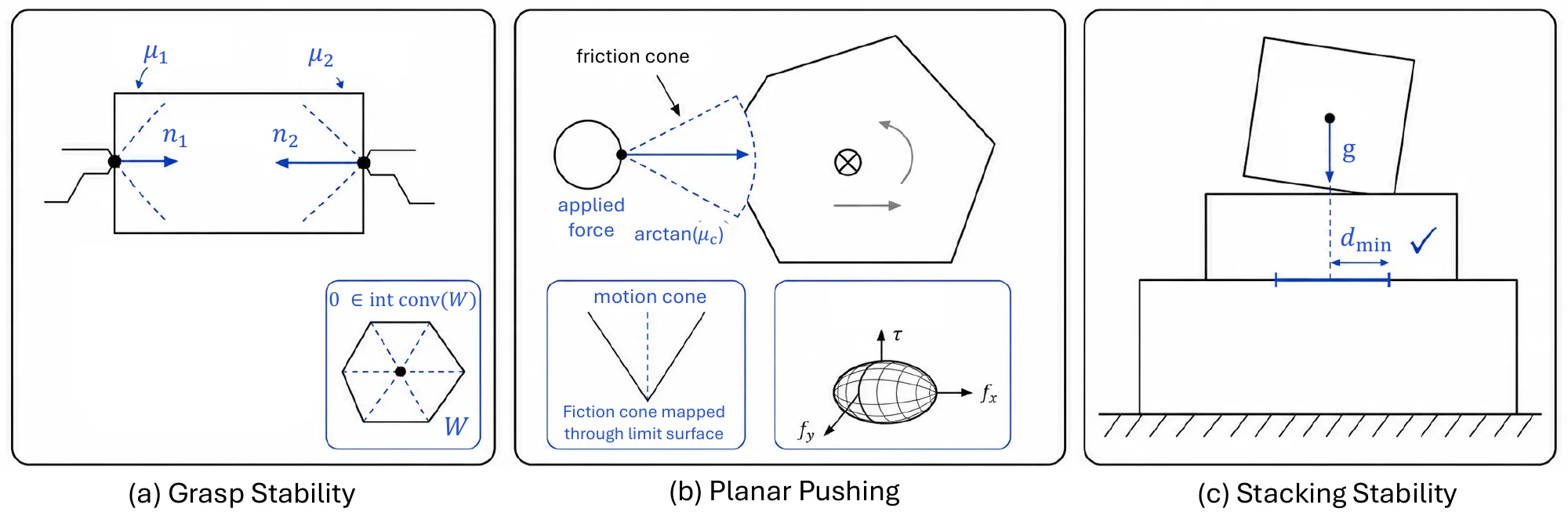
Physically-aware spatial reasoning predicts how a spatial configuration evolves under physical law: rigid-body dynamics, contact and friction, and the conditions for static stability. Will a grasp hold? How will an object move when pushed? Will a stack of blocks stand or fall? Answering these from a model of mechanics, rather than from observed correlations, is what lets a robot anticipate the outcome of an interaction before committing to it; Figure 7.2 shows the three canonical cases.
7.1.2.1Task Definition#
Let the environment at time be the state
| (7.9) |
with generalized coordinates , velocities , and physical parameters (masses and inertias in the mass matrix , friction coefficients , restitution, geometry). An action (a push, a grasp) enters as a generalized force , and the next state follows from a contact-implicit time-stepping update:
| (7.10) | ||||
where collects Coriolis, centrifugal, and gravitational terms, and for each potential contact with gap function and Jacobians the normal and tangential impulses satisfy non-penetration, complementarity, and Coulomb friction:
| (7.11) | ||||
Physical reasoning is the computation, or approximation, of this transition and of the queries derived from it (stability, collision, reachability). When motion is slow enough that inertial terms vanish, the quasi-static form
| (7.12) |
reduces reasoning to an equilibrium feasibility test, which is the setting of the classical analytic models of grasping, pushing, and stacking.
7.1.2.2Methodology#
Model-based physical reasoning is carried out either numerically, in a physics engine that integrates the dynamics above, or analytically, with closed-form criteria for the quasi-static cases. Both rest on the same Newtonian foundation and differ in whether fidelity or interpretability is the priority.
Physics Engines. MuJoCo [1187], Bullet [1188], ODE [1189], and DART [1190] integrate rigid-body dynamics with contact by time stepping, and they resolve contact in one of two ways. Penalty methods treat a contact as a compliant spring-damper that resists interpenetration,
| (7.13) |
with penetration depth , stiffness , and damping , and regularize friction similarly; they are cheap and simple, but stiff parameters destabilize the integration and soft ones introduce artificial compliance, which is acceptable in graphics and approximate planning but not in control. Constraint-based methods enforce Eq. (7.11) directly as complementarity constraints [1191], solved per step as a linear or nonlinear complementarity problem [1192], a convex quadratic program [1193], or a second-order cone program for exact friction cones [1194] (projected Gauss–Seidel and sequential-impulse schemes are the usual implementations). They give physically consistent, nearly penetration-free contact forces at higher cost and with harder scaling in the number of contacts, so engines in practice hybridize: hard constraints on normal forces, regularized tangential friction, warm starting, contact aggregation, and stabilization terms.
Analytic Quasi-Static Models. For the three settings of Figure 7.2, closed-form criteria replace simulation. At a point contact the admissible forces form the friction cone
| (7.14) |
which a polyhedral approximation turns into linear constraints. Mapping each contact’s cone through its moment arm into wrench space and taking the convex hull gives the grasp wrench space, and the grasp is force-closed when the origin lies strictly inside it, Eq. (7.8) [265]; form closure is the stronger, purely geometric condition in which contact geometry alone prevents motion, and the Ferrari–Canny -metric (the distance from the origin to the hull boundary) grades grasp quality. For planar pushing the limit surface relates the applied wrench to the resulting slip, and its ellipsoidal approximation yields a motion cone of object velocities reachable from a given push, the basis of stable pushing and closed-loop push planning. For stacking, stability under gravity requires that the gravitational wrench be balanced by the supporting contacts [1195]: without friction, the center of mass must project into the support polygon; with friction, the contacts’ friction cones must generate a wrench cone containing the gravitational wrench.
7.1.2.3Benchmarks#
PHYRE [1196] poses 2D physics puzzles in which an object must be placed so that simulated physics reaches a goal, scored by the number of attempts needed (AUCCESS) within and across puzzle templates; ShapeStacks [1195] labels 3D stacks as stable or unstable; PlasticineLab [1197] is a differentiable-physics suite for deformable manipulation; and the video suites IntPhys [1198], CLEVRER [1199], and Physion [680] test prediction and counterfactual judgment of physical outcomes, with ComPhy [1200] asking for hidden properties such as mass to be inferred from motion. Grasp quality under quasi-static analysis is evaluated on the grasping benchmarks of §7.1.1 (Cornell, YCB, GraspNet-1Billion). Metrics are predictive: position or trajectory error against the simulated outcome, success rate (stable stack, successful push or grasp), binary stability accuracy, and physical-plausibility terms such as momentum conservation and constraint violation.
7.1.2.4Challenges and Trends#
The parameters that matter most, mass, friction, elasticity, internal stability, are rarely observable. They must be inferred from interaction, from how far an object moves when pushed or how it responds to a collision; ComPhy [1200] tests exactly this, and most methods still either assume the parameters known, as classical simulation does, or approximate them in ways that fail outside the lab. Latent-dynamics learning [1201] and system identification [1202, 1203] are the two established routes.
The simulation-to-reality gap is the second limit. Small errors in restitution, micro-contact behavior, or unmodeled environmental factors compound once a policy leaves the engine, and fidelity trades against speed: high-fidelity simulation is too slow for large-scale training or real-time control, lightweight approximation too inaccurate. Hybrid physics-plus-learning models, domain adaptation between simulated and real dynamics, and uncertainty-aware transfer each address one side of this trade-off; none closes it.
Perception is the third. Geometry, material, and object state come from noisy, incomplete sensing, and a small error in shape, pose, or contact location propagates into a large error in predicted force or stability. Systems that couple vision to a physics engine, Galileo [1204] and PhyNet [1203] among them, show that physical priors improve perception and that physical consistency can constrain it in return, but end-to-end pipelines in which the two regularize each other remain the exception.
7.1.3Topological and Graph-based Reasoning#
Topological and graph-based reasoning replaces continuous geometry with discrete connectivity, so that path planning, exploration, and coordination become combinatorial search over nodes and edges: places, corridors, and routes rather than metric trajectories. The abstraction is what makes large-scale, dynamic, or partially known environments tractable, where maintaining globally consistent geometry is hard but connectivity and reachability are stable. Figure 7.3 gives the abstract formulation.
7.1.3.1Task Definition#
Given a configuration space with free subset (known a priori or inferred online from sensor streams), robot constraints, and optional priors such as floor plans or road networks, most methods build a planning graph in which vertices are places, sampled configurations, or abstract states, edges are feasible transitions, and assigns metric or semantic costs (distance, time, energy, risk); in some methods the graph is implicit and expanded locally during search. The output is a collision-free path of minimal accumulated cost, a topological map of place connectivity (often linked to local metric submaps), or, with several agents, conflict-free trajectories that minimize makespan or total cost under vertex and edge conflict constraints.
7.1.3.2Methodology#
Visibility and Line-of-Sight Graphs. Connecting configurations that can see each other reduces shortest-path planning to graph search with interpretable waypoints. The visibility graph of Lozano-Pérez and Wesley [1205] links obstacle, start, and goal vertices and recovers exact Euclidean shortest paths in polygonal environments by Dijkstra or A*; the configuration-space construction via Minkowski sums [1206] extends it to robots of finite size by growing the obstacles instead of shrinking the robot; continuous-Dijkstra algorithms settle the complexity at [1207, 1208]. Grid planners bring line-of-sight into the search itself: Field D* interpolates across cell faces for smooth, replannable paths [1209], Theta* updates parents by visibility to produce near-Euclidean paths on the fly [1210], and Jump Point Search prunes symmetric expansions by jumping between visibility events [1211].
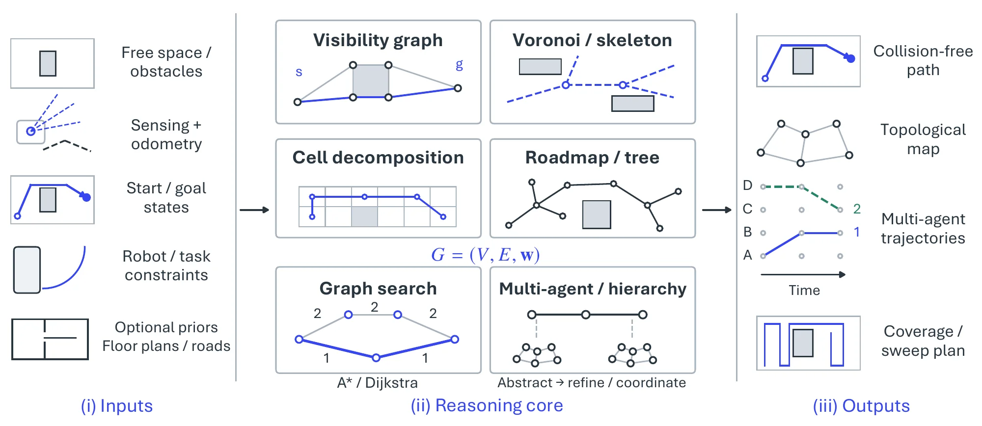
Clearance-Oriented Skeletons. Where safety matters more than length, free space is retracted to a skeleton that keeps connectivity and maximizes distance to obstacles. Voronoi diagrams and medial axes give maximal-clearance paths, with Fortune’s sweepline [1212] for efficient planar construction; the generalized and hierarchical Voronoi graphs [1213, 1214] let a robot follow ridges with its sensors and build the clearance roadmap incrementally while detecting junctions and loops; and distance-transform updates [1215, 1216] maintain the skeleton in dynamic environments for real-time replanning.
Decomposition Graphs and Coverage. Discretizing space into cells trades geometric fidelity for simplicity and completeness. Occupancy grids [79, 1217] are probabilistic cell maps updated from range data on which planning is grid search; exact decompositions serve coverage, with boustrophedon decomposition [1218] partitioning free space into monotone cells and ordering them through an adjacency graph for complete, low-redundancy sweeps; and the coverage literature is systematized in [1219].
Sampling-Based Roadmaps and Trees. In high-dimensional configuration spaces, the graph is discovered by sampling. Probabilistic roadmaps [1220] sample and connect configurations in a preprocessing phase amortized over many queries and are probabilistically complete; RRT and RRT-Connect [1221, 1222] grow trees toward unexplored regions for single-query planning under kinematic and kinodynamic constraints; PRM* and RRT* [1223] add connection-radius and rewiring rules that make them asymptotically optimal; and FMT* and BIT* [1224, 1225] combine batch sampling with dynamic programming and heuristic search over increasingly dense implicit graphs for faster, anytime convergence.
Optimal, Any-Angle, and Incremental Graph Search. On a given graph, Dijkstra’s algorithm and A* [70, 66] are the optimal single-source and heuristic searches; LPA* [1226] and D* Lite [1227] repair a shortest path incrementally as edge costs change; and the any-angle planners above (Field D*, Theta*, JPS) improve path quality without giving up the discrete search.
Multi-Agent and Hierarchical Graph Reasoning. With several agents on one graph, coordination is search over a time-expanded network. Conflict-Based Search [1228] splits the problem into a high-level search over conflict constraints and low-level single-agent planning and is complete and optimal; ICTS [1229] searches joint cost allocations backed by individual searches; ECBS and EECBS [1230, 1231] are bounded-suboptimal with focal heuristics and better conflict handling; and SAT or ILP compilations [1232, 1233] reach global optimality on moderate fleets at the cost of solver scalability. Hierarchical and multi-resolution planning [1234] and contraction hierarchies [1235] precompute abstraction layers that answer shortest-path queries on continental road networks in well under a millisecond, with standardized maps and instances [1236, 1237] for comparison.
7.1.3.3Benchmarks#
The MovingAI suite [1236, 1237] supplies standardized 2D maps from games, cities, and synthetic generators for single-agent search (path cost, runtime, memory, node expansions) and the MAPF instances on which CBS, ICTS, ECBS, and compilation-based solvers are compared by makespan, sum of costs, and success under time and memory limits, with the ICAPS MAPF tracker [1238] as the community leaderboard. OMPL’s Planner Arena [1239] compares PRM, RRT, FMT, and BIT variants on success rate, planning time, path quality, and anytime behavior, and the DIMACS shortest-path challenge [1240] evaluates query latency, preprocessing cost, and optimality on continental road graphs. Topological mapping and pose-graph SLAM are stressed by place recognition under appearance change: RADISH [1241] provides classic multi-sensor logs, and Oxford RobotCar [1242], NCLT [1243], and Nordland [1244] span seasons and weather, with KITTI and EuRoC (Section 6.2.4) for urban and indoor pose graphs.
7.1.3.4Challenges and Trends#
Graph density sets the trade-off: sparse graphs lose connectivity or optimality, dense ones lose real-time response, and the problem sharpens in high-dimensional and lifelong settings [1223, 1227]. Perceptual aliasing, drifting pose graphs, and dynamic obstacles complicate planning under partial information [54, 1245], and on the topological SLAM benchmarks the binding difficulty is not search but appearance robustness, with cross-season and cross-weather queries far harder than same-condition retrieval. Multi-agent coordination strains conflict resolution and time-expanded representations as fleets grow, while fairness and deadlock avoidance must be kept [1228, 1233, 1238].
The directions are structured rather than end-to-end: hierarchical and multi-resolution planning that abstracts and refines [1234, 1235], risk-aware and formally verified planning under uncertainty [1246, 1247], bounded-suboptimal and distributed coordination for responsiveness [1230, 1231], and neuro-symbolic methods that enrich the graph with learned perception, heuristics, and semantics [1248].
7.1.4Constraint-based Spatial Solving#
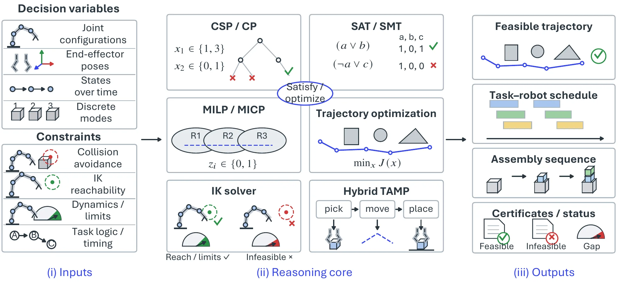
Many robotics problems are not about finding a plan but one that must satisfy strict requirements: no collisions, no joint-limit violations, stable contacts, correct timing, sometimes guaranteed dynamics or safety margins. Constraint-based spatial solving states the problem as a collection of constraints, what must hold and what must not, and hands it to a solver that either returns a satisfying solution or proves that none exists. Compared with sampling- and heuristic-driven planning, this buys certificates of feasibility, an explanation of why a candidate fails, and, under an explicit model, optimality or bounded-suboptimality guarantees, which is what manipulation in clutter, multi-robot coordination in shared space, and assembly demand. Figure 7.4 gives the abstract formulation.
7.1.4.1Task Definition#
Let collect continuous states and controls together with discrete mode and logic variables . Constraint-based solving seeks
| (7.15) |
where the inequalities encode geometric and dynamic feasibility (collision, joint, and dynamics limits), the equalities encode kinematics and contact conditions, and encodes task logic such as preconditions and effects. The optimization variant minimizes an objective as well. The output is a feasible (a collision-free and dynamically admissible trajectory, a task-robot schedule, an assembly sequence), with an objective value or optimality gap when optimizing, or a certificate that no such exists.
7.1.4.2Methodology#
The solver families differ in the variables and constraints they handle and the guarantees they return; practical systems are rarely pure, combining discrete reasoning over actions and modes with continuous optimization over motions and contacts, and calling fast geometric oracles (collision checking, inverse kinematics) inside the solver loop.
Constraint Programming (CSP/CP). When the decisions are combinatorial (which object, which placement, which grasp) but each must pass a geometric test, constraint programming encodes the choices as variables under constraints and interleaves symbolic branching with propagation, pruning, and geometric checks. Lozano-Pérez and Kaelbling [1249] cast task-and-motion planning as constraint satisfaction over action skeletons, pruning symbolic branches as soon as a geometric feasibility test fails; Lagriffoul et al. [1250] propagate and filter continuous domains before any expensive collision or IK call, so that many failures become cheap inconsistencies; and Dantam et al. [1251] interleave discrete search with incremental feasibility queries that reuse information across related constraints.
SAT/SMT Compilations. Compiling planning and feasibility into Boolean formulas, or into formulas over richer theories such as real arithmetic, puts clause learning, incremental solving, and conflict-driven pruning to work. dReal [1252] decides nonlinear real arithmetic up to a numerical tolerance (-completeness), which gives certified answers where exact decidability is impossible; SMT-based planning for hybrid systems [1253] reasons first over an abstraction and adds constraints as counterexamples appear; SAT encodings of multi-agent pathfinding [1232] obtain optimal schedules on time-expanded graphs (the MAPF problem itself is treated in §7.1.3); and SMT over linear real arithmetic extends the encodings to continuous time and to robustness against execution delays [1254, 1255].
Mixed-Integer Formulations (MICP/MILP). When discrete mode choices (which region, which contact mode, which precondition) interact with continuous geometry and dynamics, binary variables encode the nonconvex choice and convex constraints capture feasibility within a mode. IRIS [1256] inflates large convex obstacle-free regions that serve as certified safe sets, turning collision avoidance into membership constraints with explicit margins; Graphs of Convex Sets [1257] compile motion planning through clutter into a shortest-path problem over convex nodes and edges that convex optimization, with mixed-integer selection where needed, solves with certificates; and later work constructs convex sets directly in configuration space and in space-time [1258, 1259]. In each case a globally nonconvex feasibility problem is replaced by a sequence of convex ones without giving up the guarantee.
Trajectory Optimization. Even with the task fixed, an executable motion must satisfy kinematic limits, collision avoidance, smoothness, and often dynamics, which is a continuous, usually nonconvex, constrained optimization whose local optimum comes with optimality conditions and sensitivities. CHOMP [1260] deforms an initial path by functional gradient descent on a signed-distance field; STOMP [1261] replaces the gradient with stochastic perturbations to handle non-smooth costs and local minima; TrajOpt [1262] solves a sequence of convex programs with hinge-loss collision penalties; and GPMP2 [1263] writes planning as inference on a sparse factor graph with Gaussian-process priors, which gives scalability and incremental replanning. Increasingly these optimizers run inside the safe sets of IRIS and GCS, which supply initialization, constrain the search, or verify the result.
Inverse Kinematics as a Constraint Subproblem. “Is there a joint configuration that reaches this pose under limits and collisions?” is the most frequent feasibility query in any hybrid planner, so IK solvers are built as fast oracles. IKFast [1264] derives closed-form solutions and generates optimized code for repeated real-time queries; TRAC-IK [1265] combines complementary numerical strategies to raise the solve rate and avoid stalling the planner above it; and global IK by mixed-integer programming [1266] returns certifiable solutions for full chains when a feasibility proof is needed.
Hybrid Logic–Geometric Planning. In long-horizon problems the discrete decision (what to do next) and the continuous one (how to do it) cannot be separated, and task-and-motion planners close the loop between them. Logic-Geometric Programming [1267, 1268] couples symbolic action sequences to bound-constrained nonlinear programs through a multi-bound tree search, so that continuous feasibility and cost decide which symbolic branches are worth expanding; PDDLStream [1269] integrates black-box geometric generators (grasps, placements, motions) into symbolic planning by optimistic refinement, requesting continuous witnesses only when needed while remaining complete under suitable stream assumptions; R-LGP [1270] biases the search with reachability guidance; and COAST [1271] uses constraints to communicate between task planner and stream generators, cutting wasted geometric proposals by an order of magnitude in planning time.
7.1.4.3Benchmarks#
Evaluation asks whether a method returns solutions that satisfy strict feasibility conditions and, increasingly, whether it can show that it did (margins, certificates, optimality gaps) under a comparable oracle budget of collision checks and IK calls. OMPL’s benchmark suite and Planner Arena [1272] score planners on standardized problems with feasibility diagnostics and solution cost; the platform-independent TAMP benchmarks of Lagriffoul et al. [1273] specify symbolic operators together with IK and collision feasibility so that a jointly feasible task-motion plan is required; and the assembly benchmarks RAMP [1274] (real-world assemblies requiring geometric fit, stability under gravity, and grasp or fixture feasibility), ASAP [1275] (large-scale 3D assembly sequences validated by physics-based feasibility checks), and FurnitureBench [1276] (long-horizon real-world furniture assembly scored by success rate and completion time) stress feasibility across geometry, stability, and sequencing at once. Multi-robot coordination under space-time collision constraints uses the MAPF benchmarks of §7.1.3.
7.1.4.4Challenges and Trends#
The central difficulty is integrating a discrete task structure with continuous, highly nonconvex feasibility at scale and with certificates. Task-level choices (modes, grasps, placements, contact sets, schedules) interact combinatorially with geometric and dynamic constraints and fragment the feasible set; mixed-integer formulations grow expensive with the number of binary decisions [1256, 1258], trajectory optimizers return locally feasible motions that may violate a symbolic assumption such as the intended contact mode [1260, 1262], and symbolic planners propose sequences that are geometrically unrealizable. Information flows poorly in both directions: continuous solvers rarely return explanations (active sets, separating hyperplanes, -unsat cores) that the symbolic layer could use to prune, and symbolic abstractions are often too coarse to keep the continuous subproblems tractable [1269, 1267]. On the hybrid and assembly benchmarks this coupling, not raw search speed, is what separates planners: those that interleave symbolic branching with continuous oracles waste fewer feasibility checks and degrade more gracefully across domains.
Assurance under uncertainty is the second difficulty. Real systems need machine-checkable feasibility and fast infeasibility proofs, but nonlinear dynamics, contact, and hybrid interactions make strong certificates hard; convex surrogates and bounded-horizon relaxations buy speed at the price of completeness or tightness; execution requires real-time replanning with expensive oracles in the loop; and robustness to noise and model error calls for explicit risk and temporal-logic constraints [1277, 1278, 1279]. Evaluations still under-report certificate quality, oracle counts, and failure explanations.
The trend is toward structure with certificates: graphs of convex or geodesically convex safe sets that reduce global nonconvex feasibility to sequences of convex subproblems with explicit proofs [1257, 1259], coupled to trajectory-optimization and MPC back-ends that return sensitivities and constraint activations for the search above them; chance constraints, temporal logic, and control barrier functions for persistent safety [1277, 1279]; GPU acceleration for real-time replanning; and learning that guides branching, cutting, or warm starts without discarding the guarantee [1270, 1271].
7.1.5Rule-based and Programmatic Reasoning#
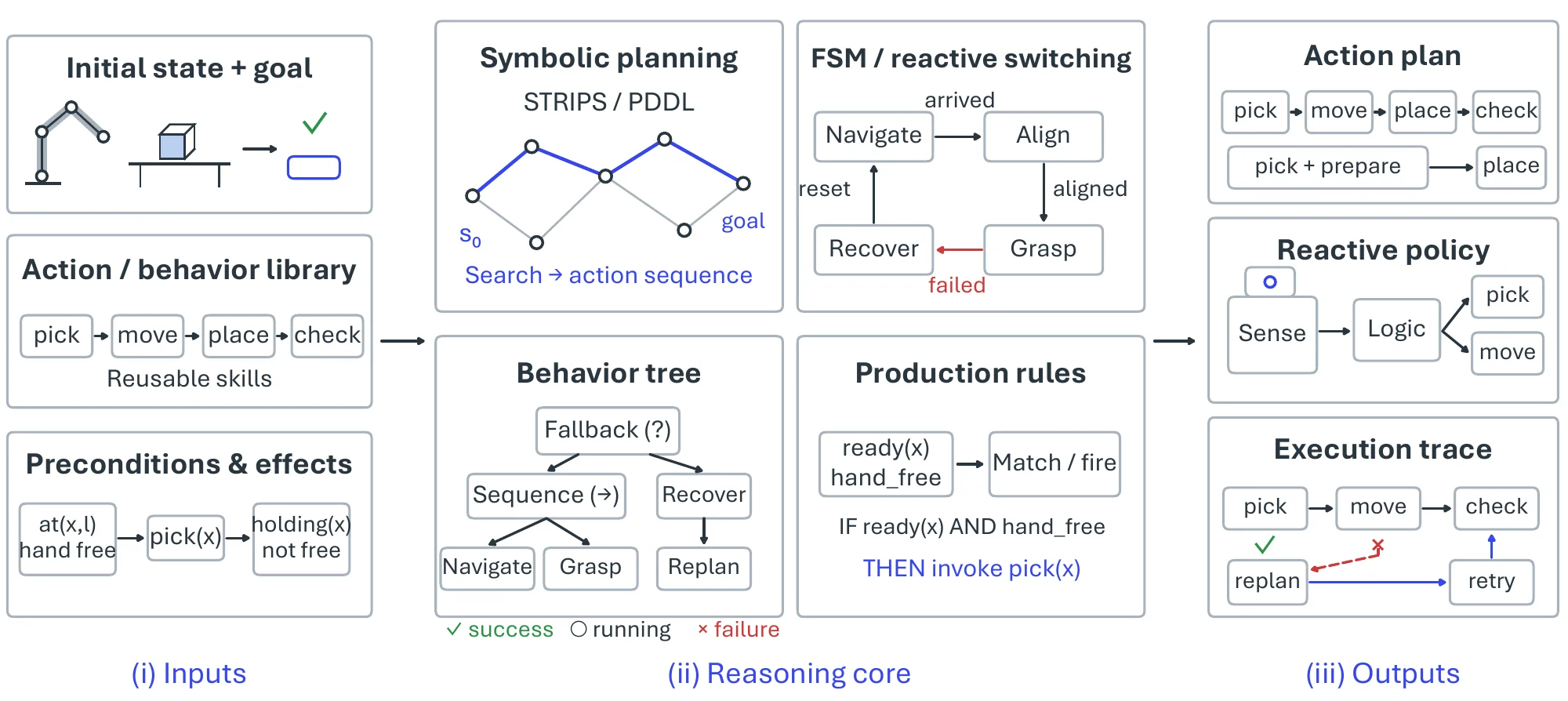
Rule-based and programmatic reasoning is the explicit, human-auditable layer that decides when an action is allowed, in what order actions happen, and what to do next when conditions change, using symbolic operators, transition rules, or program-like control structures. In a robot it is the supervisory layer that sequences reusable skills (navigate, grasp, insert) and invokes geometric solvers or learned policies only when their preconditions hold, which is what makes a decision explainable (why the detour when the corridor was blocked), verifiable, and able to carry commonsense and safety constraints through a long task. Figure 7.5 gives the abstract formulation.
7.1.5.1Task Definition#
A symbolic planning problem is a tuple with symbolic states , an operator library , an initial state , and a goal ; each operator carries a precondition and effects,
| (7.16) |
and is applicable in iff . The planning output is a sequence whose successive application to reaches a state satisfying ; the reactive variant instead returns a policy that maps the current observation and symbolic state to a behavior. Depending on the formalism, the inputs also carry resources, temporal constraints, and exogenous events.
7.1.5.2Methodology#
The formalisms split by whether they plan (search for a correct sequence before acting) or react (choose a behavior continually at run time); deployed systems usually do both, with a planner proposing the sequence and an execution structure (FSM, behavior tree, rule engine) monitoring conditions and triggering recovery.
Classical Symbolic Planning (STRIPS/PDDL and Heuristic Search). STRIPS [67] fixed the representation: planning as search over symbolic states with action schemas, so that a plan can be checked against the model and the continuous motion layer sits behind a clean abstraction boundary. PDDL [1280] standardized domain and problem specification so that planners could be compared across navigation, logistics, and assembly, with extensions (ADL, numeric fluents, temporal constructs) that capture robotic requirements without abandoning explicit semantics. Graphplan [1281] builds a planning graph whose mutual-exclusion constraints prune incompatible action combinations early, and FF [1282] made forward search fast with relaxed-plan heuristics that ignore delete effects, which capture ordering constraints such as unstacking before stacking in object-rich domains. Task-and-motion planning (§7.1.4) extends these planners with geometric feasibility checks [1283, 1284, 1285]; the common pattern is to keep the symbolic reasoning explicit, delegate feasibility to motion and IK solvers, and wrap the plan in an execution structure with monitors and recovery.
Finite-State Machines and Reactive Mode Switching. An FSM switches among a few well-defined behaviors (navigate, align, grasp) with explicit transition guards, which makes it transparent and fast but prone to state explosion as contingencies multiply. Statecharts [1286] add hierarchy and concurrency, so that complex controllers are nested reusable submachines with precise semantics; Brooks’ subsumption architecture [81] layers behaviors so that higher ones override lower ones, a blueprint for composing navigation and avoidance without global planning, systematized as behavior-based robotics [62]; teleo-reactive programs [1287] evaluate conditions continuously and fire the highest-priority satisfied rule; and ROS tooling such as FlexBE [1288] provides hierarchical, event-driven state machines at deployment scale.
Behavior Trees. A behavior tree re-evaluates its conditions on every tick and chooses among structured alternatives (sequence, fallback, parallel), so that long-horizon execution survives disturbances without committing to one fixed sequence; subtrees encapsulate reusable routines, guards and fallbacks trigger immediate recovery, and the composition semantics fit perception and motion skills. BTs originated in game AI [1289]; Marzinotto et al. [1290] formalized their semantics and their relation to other switching structures, and Colledanchise and Ögren [1291, 1292] showed which compositions preserve safety and robustness and consolidated the design principles. Compiling or wrapping a symbolic plan into a BT keeps the nominal task structure while exposing runtime guards and recovery branches [1293]; ARIAC systems pair PDDL planning with BT execution monitors to handle failures, occlusions, and defective parts [1294]; and event-driven BTs [1295] react to non-periodic stimuli rather than waiting for the next tick.
Logic-based Execution and Production Rule Systems. A production system keeps a working memory of facts and fires forward-chaining rules when their conditions hold, which suits event-condition-action policies, mode switching, and safety enforcement (no-go zones, mutual exclusions, priorities) and depends on fast incremental matching. OPS5 [1296] set the model; the Rete algorithm [1297] caches partial matches so that large rule sets update in milliseconds as facts change; CLIPS [1298] made the toolchain portable; and Soar [1299] integrated large rule bases with planning and execution in one architecture. In robotics, KnowRob [1300] and CRAM [1301, 1302] join symbolic knowledge to rule-driven execution for reasoning about actions, effects, and everyday manipulation, and LTLMoP [1303] compiles temporal-logic specifications into correct-by-construction reactive controllers whose safety and sequencing constraints are explicit at the program level.
7.1.5.3Benchmarks#
The International Planning Competition supplies the canonical PDDL domains and problems across classical, temporal and numeric, probabilistic, and HTN tracks, compared by plan quality, makespan, and runtime [1280], with planning.domains [1304] mirroring and extending the sets for reproducible evaluation. Long-horizon embodied suites test execution under partial observability and variation: BEHAVIOR-100 and BEHAVIOR-1K on OmniGibson [1305, 1306] specify household activities at the predicate level, ALFRED [1307] and TEACh [1308] score instruction-conditioned action sequences, and RoboTHOR [962] and the Habitat challenge [204] pair high-level decision logic with navigation policies under SPL. ARIAC [1294] injects faulty parts, occlusions, and failures into kitting and assembly, and FurnitureBench [1276] and RoboCup@Home [1309] stress recovery and explainability on real tasks; qualitative solvers over RCC-8 [76] and Allen relations [1310] are tested on consistency problems, and composite pipelines reuse the TAMP and OMPL harnesses of §7.1.4.
7.1.5.4Challenges and Trends#
The results on these benchmarks divide along the closed-world boundary. On IPC-style domains with fully specified preconditions and effects, classical planners remain strong; on long-horizon embodied tasks the limit is perception noise and grounding ambiguity rather than search, and a logically applicable action may be geometrically unrealizable because of a collision, an IK failure, or a missing grasp. Hand-authored operators, rules, and recovery logic also grow combinatorially with object count and contingency. Integrated task-and-motion planning (§7.1.4) answers the coupling problem by interleaving symbolic search with feasibility checks or compiling symbolic commitments into optimization back-ends [1249, 1269, 1267], and hierarchical abstraction and compositional skill models contain the search while keeping it auditable [1284, 1285].
Robustness to noise and nonstationarity is why the industrial and instruction-conditioned benchmarks reward compositions rather than single formalisms: a behavior tree around a symbolic plan makes disturbances and recoveries explicit through runtime guards, fallbacks, and safety-preserving composition [1290, 1291, 1292], and Rete-style engines [1297] supply fast event-condition-action policies over streaming facts, the pattern ARIAC entries converge on [1294].
Learned perception and language models increasingly propose the high-level procedure or heuristic while the symbolic structure stays as the safety shell that enforces preconditions, effects, and constraints: SayCan [1311] grounds language in robot skills by value-based scoring, and plan-to-BT compilation [1293] exposes parallelism, guards, and recovery at run time. Domain modeling, heuristic guidance, and recovery synthesis are being automated piece by piece while the programmatic structure is retained for auditing, debugging, and verification.
7.1.6Causal Reasoning#
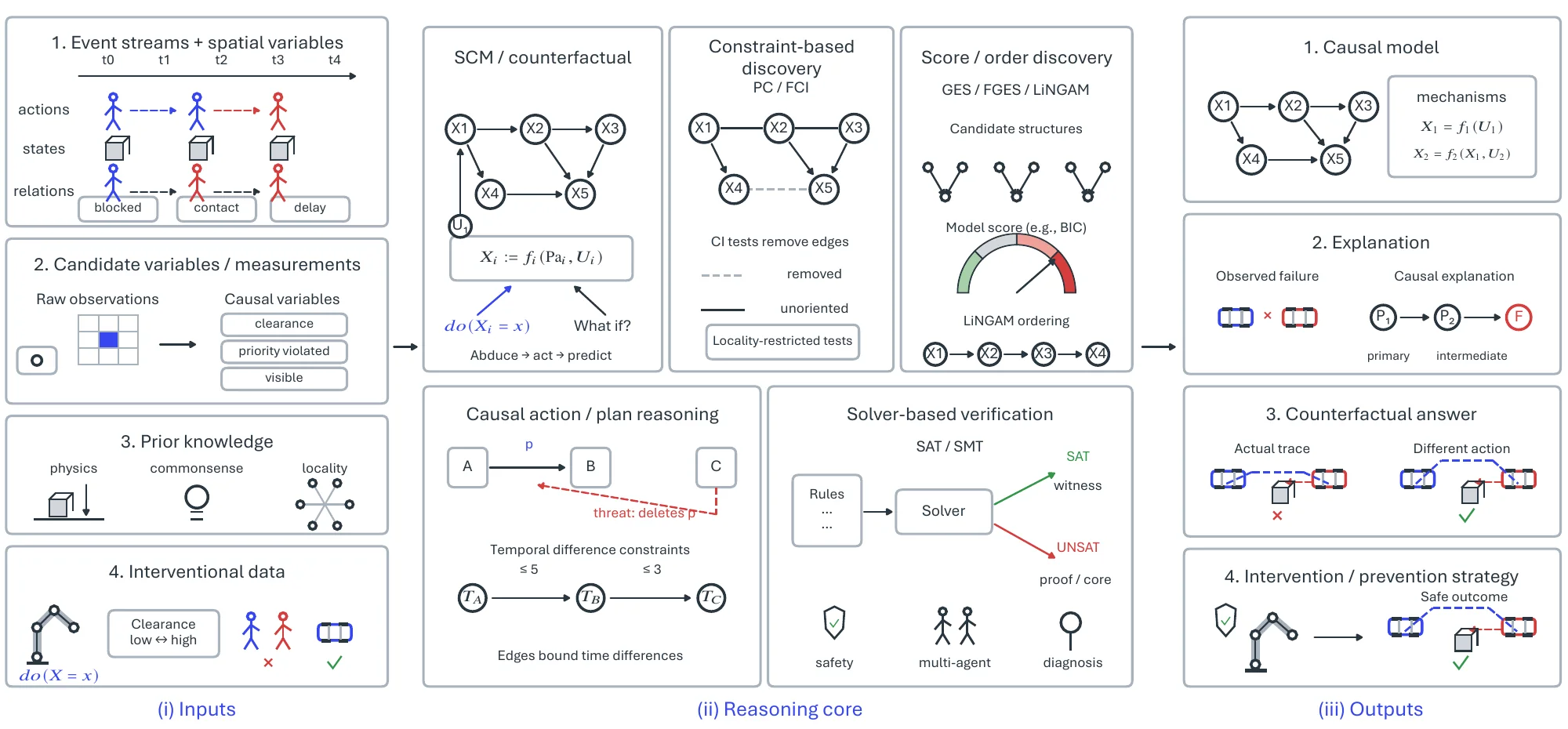
Causal reasoning moves from describing what happened to explaining why it happened and predicting what would have happened under a different action. For a robot the relevant outcomes are chains of spatial events (a collision, a delay, a deadlock, an unstable grasp, a near-miss in shared space), and making the causal assumptions explicit, rather than leaving them implicit in “actions cause state changes”, is what lets the system attribute a failure to its causes rather than its symptoms, evaluate counterfactual alternatives such as a different approach direction or timing, and, with several agents, separate primary causes from downstream effects when choosing an intervention. Figure 7.6 gives the abstract formulation.
7.1.6.1Task Definition#
The inputs are spatiotemporal event streams (agent actions, object states, contact and visibility relations, environment variables) mapped to causal variables by measurement functions (in_contact, blocked, priority_violated), optional prior knowledge from physics or commonsense, and, when available, interventional data in which a controllable variable was set deliberately. A structural causal model over these variables,
| (7.17) |
consists of a directed acyclic graph , a mechanism that generates each variable from its parents and exogenous noise , and a noise distribution [1312]. The outputs are the model itself when it must be learned, the explanation of an observed outcome (which variables caused it), the answer to an interventional query or a counterfactual one ( for a unit whose actual trace was observed), and an intervention or prevention strategy that changes controllable causes to reach a desired spatial outcome.
7.1.6.2Methodology#
The methods differ in where the causal structure comes from (assumed, learned from data, or written as domain knowledge) and in what they are asked (intervention effects, counterfactuals, responsibility, verification); in spatial domains they also differ in how they use locality, temporal precedence, and network connectivity as inductive bias.
Structural Causal Models and Counterfactuals. An SCM makes mechanisms explicit (“clearance determines collision risk”, “traffic density sets delay”) and separates intervention from observation: the operator replaces a structural equation instead of conditioning on a value, which is what is needed when, say, congestion and delay are both driven by time of day. Spatial pipelines typically start from a graph fixed by temporal precedence and locality priors (edges among nearby regions, interacting agents, adjacent cells), estimate the mechanisms from data, and validate them against implied conditional independences and refutation tests [1313]. Counterfactuals follow the abduction-action-prediction recipe: infer the exogenous noise consistent with the observed trace, apply the hypothetical intervention, predict the outcome [1312]. DoWhy and DoWhy-GCM [1314, 1315] implement identification, estimation, and refutation for this workflow on real spatiotemporal data.
Causal Discovery: Constraint- and Score-Based. When the graph is unknown but observational data are plentiful, constraint-based methods read structure off conditional independences: the PC algorithm builds the skeleton by independence tests and orients what it can, returning a Markov equivalence class, and FCI [1316] handles latent confounding and selection bias by returning a partial ancestral graph. Score-based methods instead search graph space under an objective such as BIC: GES [1317] greedily adds and then removes edges over equivalence classes, and its forward-backward structure often recovers mesoscale organization such as bottlenecks that drive downstream congestion. Spatial data strain both. Large conditioning sets are expensive and statistically weak, so practice restricts conditioning to a radius or -hop neighborhood, forbids edges that violate adjacency or reachability priors [1318], and uses order-independent variants (PC-stable [1319]) whose high-dimensional consistency is understood [1320]; ambiguous orientations are then resolved by targeted interventions. causal-learn [1321] and the TETRAD / Py-Tetrad implementations of FGES [1322, 1323] provide these pipelines at facility and city scale.
Independent-Noise Discovery (LiNGAM). In linear-Gaussian settings many edge directions are unidentifiable from independences alone. LiNGAM [1324] assumes a linear structural model with independent non-Gaussian noise, under which the causal ordering is identifiable, and DirectLiNGAM [1325] estimates it by regression rather than ICA. Spatiotemporal signals need care because autocorrelation and smoothing push the noise toward Gaussian; temporal blocking, prewhitening, and locality constraints are the usual remedies, and the recovered ordering then scaffolds an SCM for intervention analysis.
Causal Action Languages and Plan-Space Causal Links. Much causal structure in robotics is designed knowledge rather than discovered: actions have direct and indirect effects, and the system must reason about change under incomplete information. The action language C+ [1326] writes causal theories of action with inertia and nonmonotonic semantics, compactly describing how fluents such as occupied(c) or visible(a,o) evolve; CCALC [1327] compiles them to SAT or ASP so that prediction, diagnosis, and plan synthesis use the same solvers; and multi-valued fluents and external geometric predicates (collision checks, IK) are being integrated without abandoning the formal semantics [1328]. In plan space, partial-order causal-link planning [1329] represents a plan as partially ordered actions plus links (action establishes precondition for ), which makes threats explicit and repairable by promotion, demotion, or binding constraints; UCPOP [1330] extended the representation to ADL and conditional effects and VHPOP [1331] added heuristics and reachability analysis. In spatial domains a causal link is often a physical dependency, “unblock door” enabling “move cart”, which bridges symbolic causality and spatial feasibility.
Execution and Verification. A causal plan must be realized in time and checked. Simple temporal networks [1332] enforce difference constraints between events with polynomial consistency and dispatchable forms [1333], and STNUs with dynamic-controllability analysis [1334] handle contingent durations, so that ordering and clearance constraints stay satisfiable under bounded disturbance. The SAT/SMT machinery of §7.1.4 enters here as an explanation device: when a schedule is unsatisfiable, the unsat core is a minimal set of conflicting commitments, a concrete statement of which decisions caused the failure [1232, 1233]; and for hybrid dynamics -complete SMT (dReal) [1252] and dReach [1335] verify safety and synthesize interventions with numerically sound proofs or counterexamples.
7.1.6.3Benchmarks#
No single benchmark covers the causal pipeline, and the suites stress different links of it. CLEVRER [1199] pairs synthetic collision videos with descriptive, explanatory, predictive, and counterfactual questions, and CLEVRER-Humans [1336] adds human-annotated causal event graphs against which model attributions can be compared; the video suites of §7.1.2 (PHYRE [1196], Physion and Physion++ [680, 1337]) score intervention selection and latent-property inference, and CRaFT [1338], ContPhy [1339], NExT-QA [1340], AGQA [1341, 1342], and SUTD-TrafficQA [1343] ask causal questions in natural language about real and traffic video. Embodied platforms with predicate-level state (BEHAVIOR-1K, ALFRED, iGibson 2.0 [1344], ManiSkill2 [1345], RLBench [1346]; §7.1.5) test whether inferred dependencies improve intervention selection and recovery; the MAPF suites and Flatland [1347] (§7.1.3) test reasoning over space-time constraints in which one agent’s decision causes another’s delay; and ARCH-COMP [1348] with the dReal / dReach problem sets [1252, 1335] evaluate causal safety reasoning on hybrid dynamics by proof or counterexample and solve time. Discovery itself is evaluated on recovery of the Markov equivalence class under faithfulness, with scalability bounded by conditioning-set size.
7.1.6.4Challenges and Trends#
Identification is brittle. Latent confounding, selection bias, and temporal aggregation can make a query non-identifiable from logs, and estimates become unstable when locality and precedence assumptions fail [1312, 1313]; constraint- and score-based discovery is expensive on dense telemetry with strong short-range dependence and sensitive to test strength, ordering, and regularization [1316, 1319, 1320, 1317]; and LiNGAM’s non-Gaussianity is exactly what smoothed trajectories and aggregated traffic signals lack [1324, 1325]. The response is structure-aware discovery that constrains search by topology and locality and then resolves the remaining ambiguity by targeted robot interventions, connecting learning to actuation [1316, 1317].
Causal reasoning is only as good as its variables, and in embodied settings contact, occlusion, blockage, and object state must be grounded from noisy perception. The errors of that mapping propagate into SCM estimates and counterfactual conclusions [1313, 1314]. Knowledge-enabled frameworks such as KnowRob and CRAM (§7.1.5) show the shape of the interface, perception populating an explicit, interpretable model whose parameters are then estimated statistically, and the trend is toward such perception-to-symbol interfaces that tolerate sensor noise [1300, 1301, 1302].
Between a causal recommendation and a safe execution there is a verification-synthesis gap: the recommendation must become a temporally controllable schedule and a certified controller, and execution uncertainty invalidates a symbolic causal plan unless temporal networks and hybrid verification are integrated with it [1332, 1334]. SCM toolchains are therefore being embedded in decision stacks so that counterfactual policies compile into action-language or plan-space structures and then into dispatchable networks [1315, 1326, 1334], with SAT/SMT certificates and unsat-core explanations supplying the accountability [1232, 1252, 1335]; evaluation that scores explanation quality, interventional effectiveness, and certification cost on the same task is what the field still lacks.