With entities recognized and their positions fixed, what remains is how they hang together. Spatial structure construction turns independently localized entities into an organized configuration: which objects relate to which, how those relations compose into a scene, and how the scene as a whole is laid out. The section builds outward in scope, from pairwise spatial relations, through the scene graphs that assemble them, to room-level layout; it then lets structure take on time and scale, as the event structure of action detection and the whole-environment structure of mapping and SLAM. Structure in real perception is seldom purely static, and what the section yields is the explicit spatial configuration that downstream reasoning and planning act on.
6.3.1Spatial Relation Extraction#
Spatial Relation Extraction (SRE) identifies the relative spatial configuration of objects, such as “table-left of-chair” or “car-behind-bus”. It turns detections or segmentations into spatial relation knowledge that feeds reasoning, scene graph generation [776, 777, 778], autonomous driving [779, 780, 781, 782], and embodied AI [783, 784]. It is narrower than Scene Graph Generation (SGG), which runs the full pipeline from detection to relation prediction and includes non-spatial predicates (“person-holding-book”); here SRE covers only geometric, topological, and projective spatial predicates.
6.3.1.1Task Definition#
Given a visual scene (a 2D image, a video, a point cloud, or an RGB-D stream) and two target object instances specified by tags, boxes, or masks, SRE outputs their spatial relationship either as a triplet with drawn from a spatial predicate vocabulary, or as a natural-language sentence describing the relation and its context. Three subtasks differ in output granularity. Visual Spatial Classification (VSC) [785, 786] predicts the predicate from a closed label set (“on”, “in”, “next to”). Visual Spatial Description (VSD) [787, 788] generates a free-form sentence that can carry attributes and context beyond the bare predicate. Quantitative spatial understanding [789, 229] replaces qualitative predicates with metric quantities (distances, absolute sizes, 3D orientations), which navigation and manipulation require. The field has moved through these three in order, from closed-set classification to generation to metric quantification.
6.3.1.2Methodology#
Figure 6.13 summarizes the task and the three method families surveyed below.
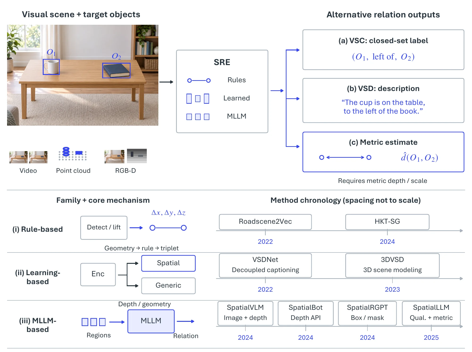
Rule-based approaches. Rule-based pipelines [779, 787, 790] first run off-the-shelf perception (a 2D detector with a bird’s-eye-view transform [791], or a 3D scene extractor [792]) to obtain each object’s 3D position, size, orientation, and appearance in a camera-centered frame whose vertical axis is aligned with gravity, and then apply deterministic geometric rules to the centroids to produce triplets [787]. Let denote the world-coordinate centroid of object , with aligned to the gravity axis. Then
| (6.34) | ||||
where is a small threshold (e.g., , m). Such rules are cheap but brittle: 2D-to-3D back-projection misplaces occluded or oddly posed objects (a rear vehicle whose centroid lands ambiguously on the BEV plane), fixed rules cannot express functional or contextual relations (“person riding bicycle”, a book more likely on a shelf than under it), and every new domain needs its rules rewritten.
MLLM-based approaches. Multimodal large language models carried the line from image-level predicates toward finer and more metric grounding. SpatialVLM [229] coupled monocular depth with the visual encoder during pre-training so the model answers metric queries such as “How far is A from B?”, outperforming GPT-4V on spatial VQA. SpatialBot [793] exposes pixel-level depth queries through a depth API and trains progressively, translating spatial reasoning into higher robotic grasping success. SpatialRGPT [789] sharpens granularity from the whole image to regions, accepting boxes or masks and auto-generating 8.7M region-level spatial samples through scene-subgraph sampling (S3). SpatialLLM [794] pairs a hybrid CLIP–DINOv2 encoder with staged data injection to hold qualitative and quantitative capabilities in one model.
6.3.1.3Datasets and Metrics#
Table 6.17 lists the benchmarks. They differ mainly in how relations were collected: manual labeling of robot-captured lab scenes in SpatialAwareRobot [795]; adversarial crowdsourcing in SpatialSense [785], where annotators propose relations that fool a baseline and only those count, which makes the dataset deliberately hard; the merge of SpatialSense and Visual Genome [796] into VSRC [787], whose 143K free-form descriptions make it the standard VSD benchmark; the 34-preposition, English–French annotations of SpatialVOC2K [797]; and the automatically generated, depth-aware SpaceSGG [776], released as 10K scene descriptions, 20K question–answer pairs, and 20K multi-turn conversations over 20K scenes.
| Dataset | Scene Type | Modality | Annotation | Samples | Relation Categories |
| SpatialAwareRobot [795] | Robotics | Image | Manual | 1,000 | 7 |
| SpatialSense [785] | Generic | Image | Manual | 11,569 | 9 |
| VSRC [787] | Generic | Image | Manual | 29,000 | 9 |
| SpatialVOC2K [797] | Generic | Image | Manual | 2,026 | 34 |
| SpaceSGG [776] | Generic | Image | Automated | 20,000 | – |
Each subtask has its own evaluation regime, and the metrics are not comparable across them. VSC is scored as classification: predicate accuracy and per-relation precision/recall on SpatialSense [785] and VSRC [787], with the driving-scene systems Roadscene2Vec [779] and HKT-SG [790] reporting per-relation F1 or accuracy on their own data; results on SpatialSense’s adversarial split lag well behind those on conventional crowdsourced data, which is the contextual-relation difficulty taken up under Challenges. VSD is scored as generation: VSDNet [787] and 3DVSD [788] report BLEU-4, METEOR, and CIDEr on VSRC, and LLaVA-SpaceSGG [776] reports QA accuracy on SpaceSGG. Quantitative understanding is the newest regime: SpatialVLM [229] and SpatialRGPT [789] report distance- and size-estimation accuracy against depth-aligned ground truth on auto-generated test sets (SpatialVLM-Bench, SpatialRGPT-Bench), SpatialLLM [794] reports combined qualitative and quantitative VQA accuracy, and SpatialBot [793] adds robotic grasp success as an embodied proxy. MLLM-based models dominate the qualitative leaderboards but still fall short on metric-scale reasoning, which motivates the unified representations discussed next.
6.3.1.4Challenges#
Spatial relations are not purely geometric. “A cup on a table” is plausible and “a cup on a wall” is not, yet the two differ only in object identity, so rule-based and purely geometric methods cannot capture functional or commonsense constraints; a model needs to know what objects are for and where they tend to be, not just their boxes or point coordinates. Metric grounding is the second gap. MLLMs handle contextual and functional predicates well but judge distances, sizes, and angles poorly; injecting geometry and depth during pre- or post-training, or exposing dedicated spatial tools, is the current route, and the longer-term goal is a representation that holds discrete predicates (“near”) and continuous quantities (“2 meters away”) together, since navigation and manipulation need both. Generalization is the third. SpatialSense [785] and VSRC [787] cover a small slice of real scenes, and models trained on them degrade under new object appearances, scene complexity, lighting, and occlusion; SpatialVLM [229] and its successors generalize better, but unseen and dynamic environments remain largely untested.
6.3.2Scene Graph Generation#
Scene graph generation (SGG) [798, 799, 800] parses visual content into a graph of triplets, each joining a subject and an object through a predicate, for example . The graph records not only which objects are present but how they interact, which is what retrieval [598, 801], captioning [802, 803], autonomous driving [804, 805, 779], and robotics [806, 807, 808] consume downstream.
6.3.2.1Task Definition#
Given a visual scene, SGG produces a graph
| (6.35) |
where each entity in is an object instance with a localization (a bounding box, or a mask in the panoptic setting) and a class label, and is a predicate from a relation vocabulary describing how and interact.
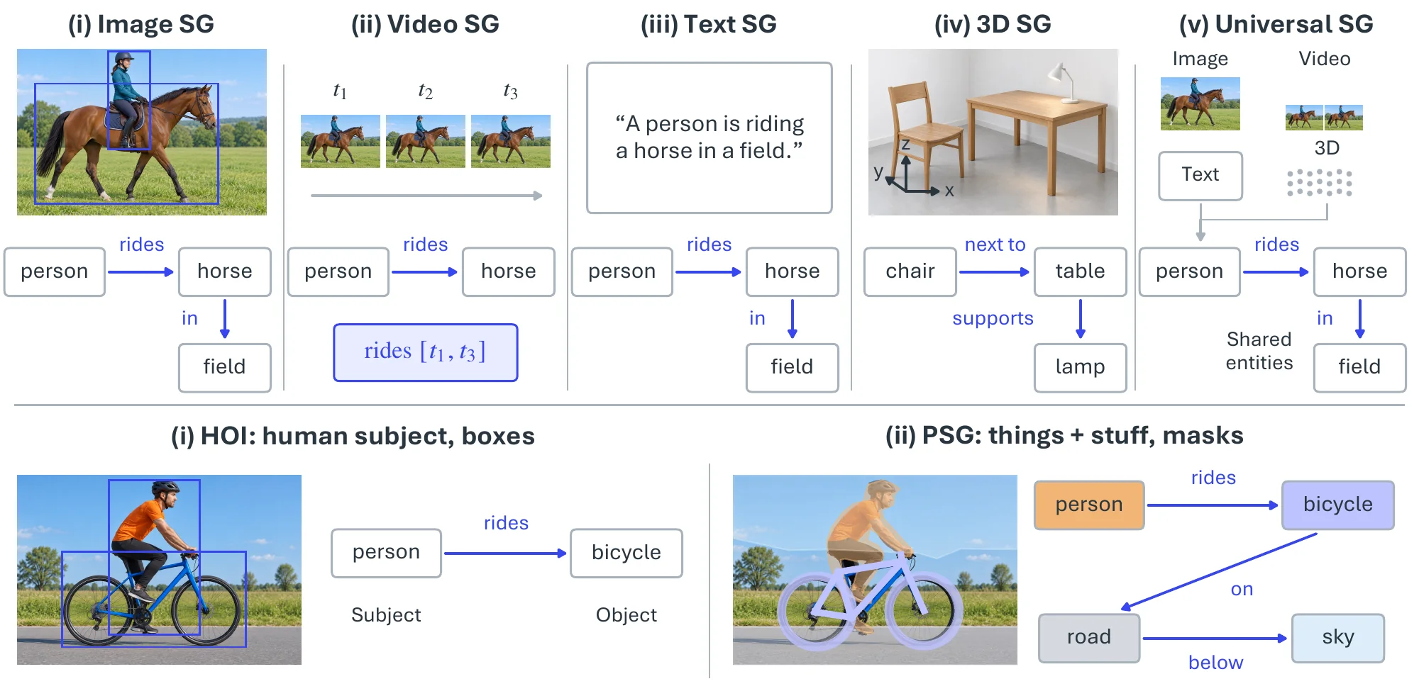
The task is instantiated by input modality. Image SGG (ISG) [796, 809] on static 2D images is the original and most studied setting and anchors most benchmarks. Video SGG (VSG) [810, 811] adds time, so relations become dynamic and temporally extended, and temporal context disambiguates interactions a single frame leaves open. Textual SGG (TSG) [812, 813] parses a sentence (“A person is riding a horse in a field”) into a graph, treating SGG as structured language parsing. 3D SGG (3DSG) [342, 343] operates on point clouds or meshes and models relations in metric 3D space, free of the perspective ambiguity of images. Universal SGG (USG) [778] aims at one graph from several simultaneous modalities (image, video, 3D, text). Two further variants change the level of detail rather than the modality. Human–Object Interaction detection (HOI) [814, 815] restricts the subject to humans and has become a field of its own because of pose variability and the subtlety of intent. Panoptic SGG (PSG) [816, 817] grounds nodes on panoptic segmentation masks instead of boxes, so relations can involve “stuff” (sky, road) and are localized without the imprecision of boxes.
6.3.2.2Methodology#
Figure 6.14 illustrates the five modality settings and the two specializations with a representative input and output each.
Two-stage methods. Two-stage methods [798, 809, 818, 819, 820, 821] were the standard for years: a pre-trained detector such as Faster R-CNN [172] produces boxes and per-object features, and a separate relation model predicts a predicate for each pair. Specializing each stage made the graphs accurate, but detector errors propagate uncorrected into relation prediction, the two models are trained and tuned separately, and object interactions are only modeled after detection has already committed.
One-stage methods. One-stage methods [822, 823, 824, 825] fold detection and relation prediction into one end-to-end network. Pixel-based [824] and fully convolutional [825] formulations came first; after DETR [136], most one-stage SGG adopted set prediction with learned queries, and the methods differ in what the queries represent. RelTR [826] uses paired subject–object queries so the Transformer predicts relations between pairs directly; SGTR [827] decouples subject, object, and predicate queries and composes them, which lets each component be predicted on its own; and PSGTR [816] uses triplet queries that emit scene-graph triplets without a detector at all.
Prior knowledge. Because predicates are long-tailed and many relations are not visually decidable, SGG has long imported priors. Language priors [828, 829, 830] supply semantic embeddings that help rare predicates; statistical priors [831, 832, 821] model object-pair co-occurrence; knowledge graphs such as ConceptNet [833] add commonsense [834, 835]; and LLMs bring world knowledge [836, 837].
Beyond images. The non-image settings reuse these designs and add modality-specific machinery. Video SGG tracks object tubes and aggregates relations over time: TRACE [810] decomposes relation prediction by temporal segment and STTran [811] applies a spatio-temporal Transformer over frame-level graphs. Textual SGG is a parsing problem, for which the FACTUAL parser [812] fine-tunes a sequence-to-sequence model to emit faithful triples. 3D SGG predicts relations from point-cloud or mesh segments with graph networks [342], and SceneGraphFusion [343] does so incrementally from an RGB-D stream so the graph grows with the reconstruction. Panoptic SGG is served by the triplet-query PSGTR [816] and its video extension [817], and USG [778] shares one graph decoder across image, video, 3D, and text inputs.
6.3.2.3Datasets and Metrics#
| Dataset | Modality | Obj. Class | BBox | Rela. Class | Triplets | Instances |
| Visual Phrase [838] | Image | 8 | 3,271 | 9 | 1,796 | 2,769 |
| Scene Graph [598] | Image | 266 | 69,009 | 68 | 109,535 | 5,000 |
| VRD [829] | Image | 100 | - | 70 | 37,993 | 5,000 |
| Open Images v7 [442] | Image | 600 | 3,290,070 | 31 | 374,768 | 9,178,275 |
| Visual Genome [796] | Image | 5,996 | 3,843,636 | 1,014 | 2,347,187 | 108,077 |
| GQA [839] | Image | 200 | - | 310 | - | 3,795,907 |
| VrR-VG [840] | Image | 1,600 | 282,460 | 117 | 203,375 | 58,983 |
| UnRel [841] | Image | - | - | 18 | 76 | 1,071 |
| SpatialSense [785] | Image | 3,679 | - | 9 | 13,229 | 11,569 |
| SpatialVOC2K [797] | Image | 20 | 5,775 | 34 | 9,804 | 2,026 |
| OpenSG [816] | Image (panoptic) | 133 | - | 56 | - | 49K |
| AUG [842] | Image (overhead) | 76 | - | 61 | - | - |
| STAR [843] | Image (satellite) | 48 | 219,120 | 58 | 400,795 | 31,096 |
| ReCon1M [844] | Image (satellite) | 60 | 859,751 | 64 | 1,149,342 | 21,392 |
| SkySenseGPT [845] | Image (satellite, instruction) | - | - | - | - | - |
| Traffic Scene Graph [804] | Image (traffic) | 2,266 | - | 4,272 | - | 451 |
| ImageNet-VidVRD [846] | Video | 35 | - | 132 | 3,219 | 100 |
| VidOR [847] | Video | 80 | - | 50 | - | 10,000 |
| Action Genome [848] | Video | 35 | 0.4M | 25 | 1.7M | 10,000 |
| AeroEye [849] | Video (drone) | 56 | - | 384 | - | 2.2M |
| PVSG [817] | Video (panoptic) | 126 | - | 57 | 4,587 | 400 |
| ASPIRe [850] | Video (interlacements) | - | - | 4.5K | - | 1.5K |
| Ego-EASG [851] | Video (egocentric) | 407 | - | 235 | - | - |
| IESG [805] | Video (traffic) | 9 | - | 16 | - | - |
| 3DSSG [342] | 3D | 528 | - | 39 | - | 48K |
| PSG4D [852] | 4D | 46 | - | 15 | - | - |
| 4D-OR [853] | 4D (operating room) | 12 | - | 14 | - | - |
| MM-OR [854] | 4D (operating room) | - | - | - | - | - |
| EgoExOR [855] | 4D (operating room) | 36 | - | 22 | 568,235 | - |
| TSG Bench [856] | Text | - | - | - | 11,820 | 4,289 |
| FACTUAL [812] | Text, Image | 4,042 | - | 1,607 | 40,149 | 40,369 |
| DiscoSG-DS [857] | Text, Image | 4,018 | - | 2,033 | 68,478 | 8,830 |
Table 6.181 lists the benchmarks by modality. The image benchmarks run from the small precursors Visual Phrase [838], Scene Graph [598], and VRD [829], which first exposed the long-tailed predicate distribution, to Visual Genome [796], Open Images [442], and GQA [839], with VrR-VG [840] and UnRel [841] carved out to test visually relevant and zero-shot relations respectively. Visual Genome is the primary benchmark but its raw release (33,877 object and 40,480 relationship synsets) is noisy and heavily long-tailed, so the community works with cleaned subsets: the broad cleaning in Table 6.18 keeps roughly 6K object and 1K predicate classes, and the de-facto SGG benchmark VG150 restricts these to the 150 most frequent object and 50 most frequent predicate classes. Spatial-only relations are covered by SpatialSense and SpatialVOC2K (see the preceding subsection), panoptic grounding by OpenSG [816], and non-standard viewpoints by the overhead AUG [842], the satellite STAR [843], ReCon1M [844], and instruction-based SkySenseGPT [845], and the traffic-scene graphs of [804]. Video benchmarks began with ImageNet-VidVRD [846] and the trajectory-annotated VidOR [847], then specialized to human activity (Action Genome [848]), drone footage (AeroEye [849]), panoptic video (PVSG [817]), fine topological interlacements (ASPIRe [850]), egocentric capture (Ego-EASG [851]), and imminent traffic events (IESG [805]). 3DSSG [342] is the standard 3D benchmark; PSG4D [852] adds time, and the operating-room sets 4D-OR [853], MM-OR [854], and EgoExOR [855] bring multimodal (RGB-D, audio, robot logs) and egocentric surgical scenes. On the text side, TSG Bench [856] evaluates LLMs on graph generation from narratives, while FACTUAL [812] and DiscoSG-DS [857] pair images with text for factually consistent, cross-modal graphs.
Evaluation separates what is given from what is predicted. In Predicate Classification (PredCls) boxes and object labels are given and only predicates are predicted; in Scene Graph Classification (SGCls) boxes are given and both object labels and predicates are predicted; in Scene Graph Generation (SGGen, also SGDet) everything is predicted, and a triplet counts only if both boxes overlap their ground truth at IoU , with Phrase Detection relaxing this to the union box and SGGen+ also crediting correctly detected singleton nodes. Panoptic SGG replaces box IoU with mask IoU. The standard metric is recall of ground-truth triplets among the top- predictions,
| (6.36) |
under a graph constraint (one predicate per pair) or without it. Because is dominated by frequent predicates, mean Recall@K () averages recall per predicate class and has become the long-tail metric of record; the gap between and drove much of the debiasing literature [819, 818, 821]. Weighted triplet recall, micro- versus macro-averaging over images, the stricter / of the Open Images challenge, and retrieval-based R-Precision are reported in specific settings.
Each modality has its own benchmark and protocol, so leaderboards are not comparable across types: video SGG uses ImageNet-VidVRD, VidOR, and Action Genome with the same triad plus temporal-IoU thresholds; textual SGG uses set F1 over triples on FACTUAL and LLM-judged action coverage on TSG Bench; 3D SGG uses object-, predicate-, and triplet-level recall on 3DSSG; panoptic SGG uses mask-IoU on OpenSG and PVSG. Table 6.19 therefore reports only the image setting, where VG150 SGDet is shared.
| Method | Family / backbone | Year | R@50 | R@100 | mR@50 | mR@100 |
| Neural Motifs [809] | Two-stage, X-101-FPN | 2018 | 32.1 | 36.9 | 5.5 | 6.8 |
| BGNN [818] | Two-stage, X-101-FPN | 2021 | 31.0 | 35.8 | 10.7 | 12.6 |
| SGTR [827] | One-stage, DETR-R101 | 2022 | 24.6 | 28.4 | 12.0 | 15.2 |
| RelTR [826] | One-stage, DETR-R50 | 2023 | 27.5 | – | 10.8 | – |
| EGTR [822] | One-stage, Deformable DETR-R50 | 2024 | 30.2 | 34.3 | 7.9 | 10.1 |
Table 6.19 shows the trade-off that still shapes image SGG. The two-stage Motifs baseline keeps the highest overall recall, but its mean recall is the lowest, which is the frequent-predicate bias in numbers; BGNN’s debiasing doubles mean recall at a small cost in . The one-stage DETR-style models start several recall points lower, since they must detect and relate in one pass with a weaker backbone, yet SGTR and RelTR reach the best mean recall of the group, and EGTR closes most of the overall-recall gap to two-stage methods while running end to end.
6.3.2.4Challenges#
From single-modality to universal SGG. Methods are built per modality, yet real scenes are multimodal, with images carrying visual detail and text carrying abstract concepts and events. A universal scene graph [778] would express all of them in one cross-modal representation; the hard part is identifying the same objects, events, and relations across modalities and suppressing cross-modal noise, and granularity has to follow the application rather than a fixed ontology, since robotic interaction or driving may need relations at a level of detail that image-level graphs do not provide.
Integrating SGG with MLLMs. MLLMs are strong at language and weaker at structured visual understanding. Scene graphs offer a way in: pretraining objectives that mask and predict graph nodes (objects, attributes, relations) across image, video, and text inputs would teach a language model to read structure rather than only the next token, and the scene-graph-guided MLLMs of the preceding subsection [776] are an early instance.
From images to embodied use. Most SGG analyzes static images or videos, but the graph is most useful when it is kept live: robots update it as they act [806, 807, 808], and driving systems read relations among lanes, signs, and pedestrians from it [804, 805, 779]. As these uses grow, the scene graph shifts from a product of perception to the state on which decision and interaction operate.
6.3.3Layout Estimation and Room Parsing#
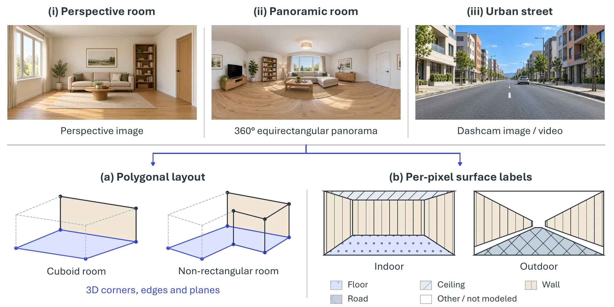
Layout estimation recovers the structural geometry of an indoor space, the corners, walls, floor, and ceiling that bound it, as a simplified 3D “wireframe” called the room layout. Room parsing extends this by also detecting, localizing, and labeling the objects inside (furniture and fixtures), giving a complete description of the scene. For outdoor scenes, the analogous problem is recovering a road layout in bird’s-eye view from a street image [858]. Figure 6.15 shows the inputs and output representations for the structural part of the task.
6.3.3.1Task Definition#
Given an image (a perspective view, a panorama, or a multi-view or video capture), layout estimation recovers the dominant surfaces that bound the navigable volume of a room as a room layout , where each is a planar polygon in 3D; equivalently the output may be plane parameters or a per-pixel structural-surface label map. Under a vertical-wall model, the layout compresses to a floor-plan polygon with floor and ceiling heights . Outdoor road-layout methods instead predict road regions and vehicle occupancy in bird’s-eye view. Room parsing adds per-object instance masks or boxes with class labels, drawn from a fixed ontology or, in the open-vocabulary setting, from free-form language.
6.3.3.2Methodology#
Pre-deep-learning approaches. Classical room layout estimation rests on the Manhattan assumption [8]: the scene is built from surfaces aligned with three mutually orthogonal directions, as walls, floors, and ceilings in most built environments are. Hedau et al. [859] introduced the task, modeling a cluttered indoor image jointly as a 3D box layout (the room as if empty) and per-pixel surface labels (visible walls, floor, ceiling, and objects). Three mutually orthogonal vanishing points are first estimated with a robustified variant of Rother’s method [860], in which a line segment votes for a candidate vanishing point with
| (6.37) |
where is the angle between and the line from the midpoint of to , is the segment length, and is a fixed bandwidth; candidates are selected greedily, removing the lines that supported each selected point. The vanishing points fix the orientation of the box; sampling pairs of rays through two of them generates box-layout hypotheses, whose remaining edges follow from the third vanishing point, and a learned structured regressor scores the hypotheses and selects the layout.
Deep learning approaches. Mallya and Lazebnik [861] first used a fully convolutional network to predict informative edge maps, then kept the classical hypothesis-generation-and-ranking step, scoring hypotheses with features from the learned edges together with line membership and geometric context. Later deep estimators are best organized by input modality and geometric representation, which vary independently: panorama input does not imply a cuboid output, and non-cuboid geometry need not break the Manhattan assumption. Figure 6.16 groups the representative methods of 2015–2021 along these lines.
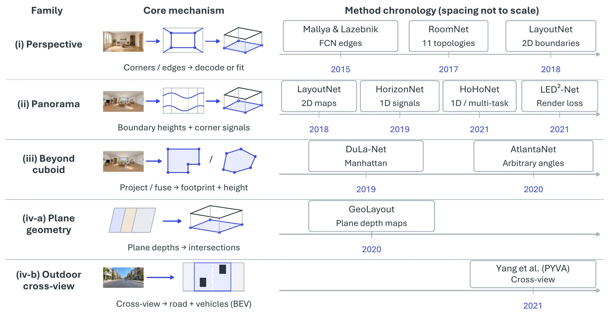
(i) Perspective-image corner and edge predictors. RoomNet [862] regresses an ordered set of room corners with a recurrent encoder–decoder conditioned on one of 11 predefined cuboid topologies, and LayoutNet [863] predicts corner and boundary probability maps and fits a cuboid to them. The topology constraint simplifies reconstruction, but a single perspective view often leaves part of the room outside the frame.
(ii) Panorama-based methods. A equirectangular panorama removes the field-of-view truncation of a perspective image, though not occlusion. LayoutNet [863] predicts 2D corner and boundary maps from a gravity-aligned panorama; HorizonNet [864] compresses the layout into three 1D per-column signals (floor-wall boundary, ceiling-wall boundary, and wall-wall corner indicator), adds Pano Stretch augmentation, and reconstructs general Manhattan layouts as well as cuboids; HoHoNet [865] learns latent horizontal features decodable into layout, depth, and semantics; and LED2-Net [866] supervises the layout through differentiable depth rendering, comparing depth rendered from the predicted layout with the target geometry.
(iii) Beyond-cuboid and Atlanta-world methods. Floor-plan prediction separates the number of walls from the constraints on their orientation. DuLa-Net [867] combines equirectangular and ceiling–floor projections to estimate a floor plan under a Manhattan prior, which admits non-rectangular rooms with orthogonal walls. AtlantaNet [868] projects a gravity-aligned panorama onto horizontal planes above and below the camera and predicts a room footprint and height under the Atlanta-world model, which keeps walls vertical but allows arbitrary horizontal orientation, including curved footprints. Both still assume vertical walls, so slanted walls and ceilings remain out of reach.
(iv) Plane-based indoor geometry and outdoor cross-view prediction. GeoLayout [869] predicts pixel-level plane parameters, infers the depth map of each dominant plane, and reads layout boundaries off the intersections of those depth maps, a geometric alternative to regressing polygon vertices; the accompanying Matterport3D-Layout dataset covers cuboid and non-cuboid rooms. For outdoor scenes, Yang et al. [858] use a cross-view transformation with cycle-consistency constraints to predict road layout and vehicle occupancy in bird’s-eye view from a monocular front-facing image.
6.3.3.3Datasets and Metrics#
Table 6.20 summarizes the benchmarks. Perspective-image evaluation grew from Hedau [859] (308 web and LabelMe images with box layouts and surface labels) through its augmented successor Hedau+ and the more cluttered SUNbox drawn from SUN2012 [607], both built by Mallya and Lazebnik [861] to train FCN edge predictors, to LSUN Room Layout [870], the standard perspective benchmark with corner positions and cuboid topologies on over 5K images. Corridor and video data serve navigation: Yang [871] labels ground versus wall in corridor images, FreeYourCamera [872] records six-degree-of-freedom smartphone walks that frequently violate box and Manhattan assumptions, and MichiganIndoorCorridor [873] provides non-Manhattan corridors with glass and reflections. Panoramic and 3D evaluation rests on PanoContext [874] (cuboid layouts and furniture for about 500 SUN360 panoramas, the standard testbed for LayoutNet, HorizonNet, and LED2-Net), Stanford 2D-3D-S [875] (about 70K RGB-D panoramas with depth, normals, semantics, and meshes over 270 rooms, enabling joint layout-depth-semantics evaluation), and Matterport3D-Layout [869], derived from Matterport3D [340] with RANSAC-fitted plane ground truth for cuboid and non-cuboid rooms.
| Dataset | Year | Scene | Modality | Scale | Annotation |
| Hedau [859] | 2009 | Room | Image | 308 | Box layout + surface labels |
| Hedau+ [861] | 2015 | Room | Image | 337 | Box layout (Hedau + 75 bedroom images) |
| SUNbox [861] | 2015 | Room | Image | 543 | Box layout, cluttered SUN2012 scenes |
| LSUN Room Layout [870] | 2015 | Room | Image | 5,394 | Corners + 11 cuboid topologies |
| Yang [871] | 2016 | Corridor | RGB-D image | 967 | Ground / non-ground masks |
| FreeYourCamera [872] | 2013 | Mixed | Video (6-DoF) | 10 seq. (84 frames) | Layout under non-box, non-Manhattan motion |
| MichiganIndoorCorridor [873] | 2011 | Corridor | Video | 11 seq. (3,300 frames) | Ground + three walls on first frame |
| PanoContext [874] | 2014 | Room | Panorama | 500 | Cuboid layout + furniture |
| Matterport3D-Layout [869] | 2020 | Room | RGB-D image | 7,360 | Plane parameters, cuboid + non-cuboid |
| Stanford 2D-3D-S [875] | 2017 | Building | RGB-D panorama | 70K | Layout, depth, normals, semantics, mesh |
Metrics follow the output representation. Perspective benchmarks (Hedau, LSUN) report pixel error, the fraction of pixels whose predicted surface label differs from the ground truth, and corner error, the mean distance between predicted and true corners normalized by image size; the edge-map methods additionally report the contour-detection F-scores at the optimal dataset scale (ODS, one threshold for the whole set) and optimal image scale (OIS, the best threshold per image). Panoramic and 3D benchmarks (PanoContext, Stanford 2D-3D-S, Matterport3D-Layout) report 3D and 2D room IoU between the predicted and ground-truth layout volumes or floor plans, with frequency-weighted IoU and pixel accuracy as segmentation-style complements. A method trained for one input type rarely transfers to the other without re-training, so perspective and panoramic results are not compared directly, and the outdoor road-layout protocol [858] is separate again.
| Method | Representation | Year | PanoContext | Stanford 2D-3D-S | Matterport3D-Layout |
| LayoutNet [863] | 2D corner + boundary maps | 2018 | 74.48 | 76.33 | 75.82 |
| DuLa-Net [867] | Dual projection, Manhattan plan | 2019 | 77.42 | 79.36 | 75.05 |
| HorizonNet [864] | 1D column representation | 2019 | 82.17 | 79.79 | 78.73 |
| AtlantaNet [868] | Top-down footprint, Atlanta world | 2020 | 78.76 | 82.43 | 80.02 |
| LED2-Net [866] | Differentiable depth rendering | 2021 | 82.75 | 83.77 | 81.52 |
Table 6.21 compares the panorama methods under one protocol. The 1D column representation of HorizonNet gained about eight IoU points over LayoutNet’s 2D maps on PanoContext, and the geometric supervision of LED2-Net adds a further point or two on every benchmark; the beyond-cuboid methods pay for their generality on cuboid-heavy PanoContext (DuLa-Net, AtlantaNet below HorizonNet) and recoup it on Matterport3D-Layout, whose non-cuboid rooms are exactly what they were designed for.
6.3.3.4Challenges#
The geometric priors that make layout estimation tractable also bound it. Cuboid models cannot express alcoves or L-shaped plans; Manhattan models keep orthogonal walls even when the footprint is free-form; the Atlanta-world model of AtlantaNet [868] frees wall orientation but not wall tilt; and plane-based methods such as GeoLayout [869] approximate curved geometry only with many planes. Slanted enclosures, split levels, and the outdoor bird’s-eye-view target of [858], which is a different output space altogether, all sit outside the standard formulations. Clutter and occlusion are the second obstacle: furniture hides the corners, boundaries, and vanishing lines that both classical and learned methods read, so estimators must hallucinate hidden structure from layout priors, and confidently wrong boundaries without uncertainty are the typical failure. Generalization follows from the data: benchmarks are indoor, mostly rooms and corridors, and models trained on one set degrade on another’s appearance, architecture, and lighting, while sparse, unposed multi-view capture breaks the pose assumptions of classical pipelines; the feed-forward geometry models of §6.2.4 are the natural starting point for layout from such input.
6.3.4Action Detection#
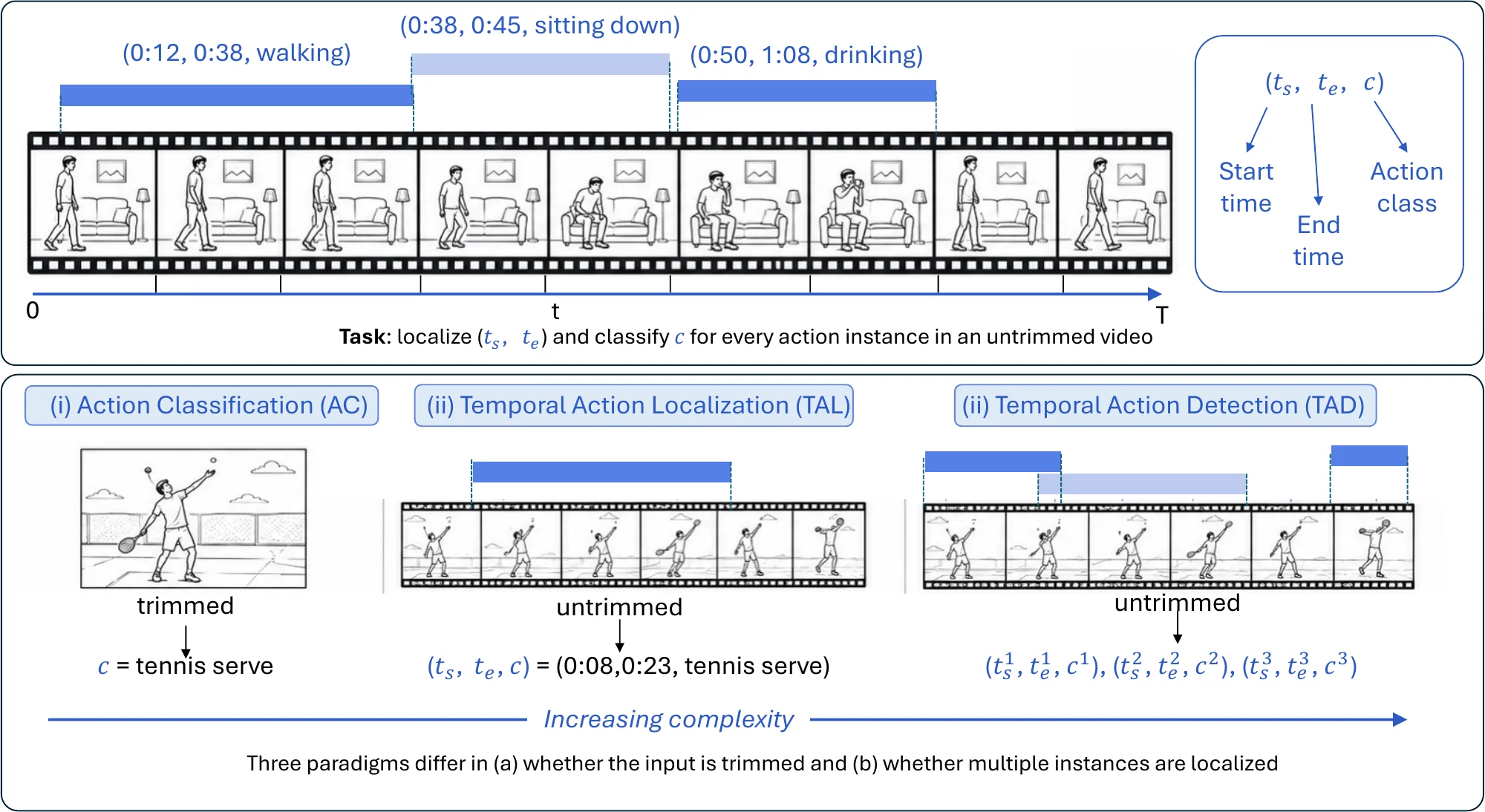
Action detection (AD) finds human actions in untrimmed video: for each action instance it returns the time interval in which it occurs and its category . Where action recognition classifies a clip that has already been trimmed to one action, detection must also decide when actions start and end, in streams that contain many of them. It belongs to spatial structure construction because it organizes the entities and relations of a scene along the time axis into events, the temporal counterpart of the scene graphs above and the basis of video SGG and human–object interaction. Figure 6.17 illustrates the task.
6.3.4.1Task Definition#
Given an untrimmed video (or a continuous multi-sensor stream), AD outputs a set of tuples with start time, end time, and category for every action instance. Three settings differ in what is assumed about the input. Action classification (AC) takes a trimmed clip and predicts one category, with no localization. Temporal action localization (TAL) predicts start and end times in untrimmed video, usually assuming one dominant action per video. Temporal action detection (TAD) is the general case: multiple instances per video, possibly overlapping or concurrent, across temporal scales, each to be localized and classified.
6.3.4.2Methodology#
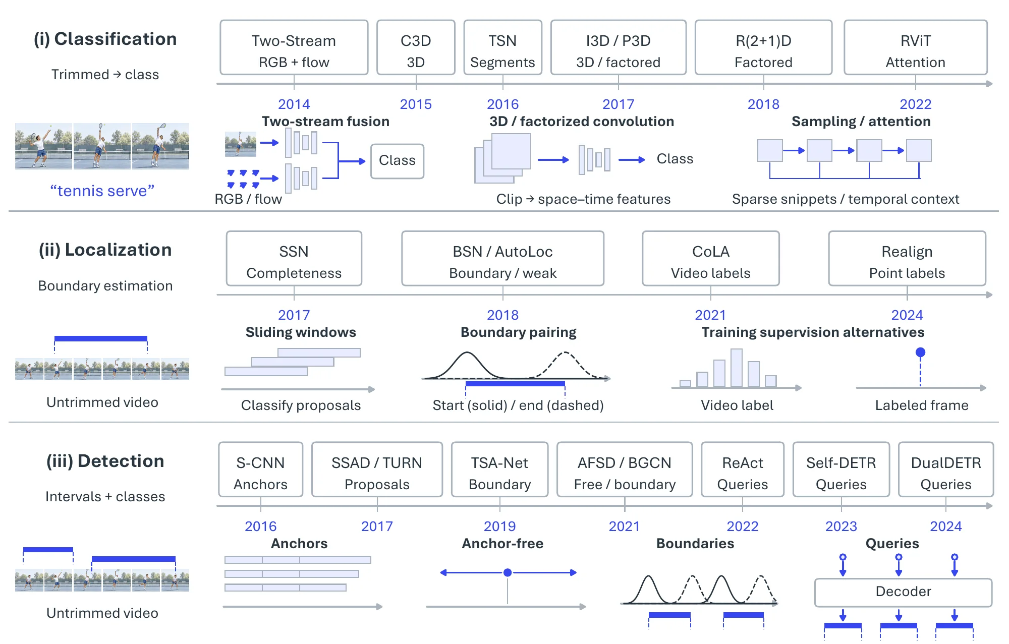
Figure 6.18 organizes the methods by the three settings; each builds on the previous one’s representations.
Action Classification. Two-stream CNNs [876] model appearance from RGB frames in one stream and motion from dense optical flow in another, fusing the two at the output. 3D CNNs [877] convolve over space and time jointly, C3D [238] and I3D [239] being the standard examples, at the cost of a large parameter count that R(2+1)D [878] and P3D [879] reduce by factoring 3D convolution into 2D spatial and 1D temporal steps. TSN [880] samples a few snippets sparsely across a long video and supervises at video level, which scales long-range temporal modeling cheaply, and Transformers [881, 882] model global spatio-temporal dependencies among sampled tokens beyond the local reach of convolution.
Temporal Action Localization. Early TAL ran a classifier over dense, fixed-size sliding windows, which was both slow and blind to the wide range of action durations. Structured segment networks [883] instead model a proposal’s starting, ongoing, and ending stages and score its completeness, which refines boundary regression. Boundary-sensitive methods [884] go further and predict start and end probabilities at every snippet, then pair high-confidence boundary points into proposals; this flexible boundary generation is the component on which later detection systems rest.
Because precise boundary annotation is expensive, weakly supervised TAL (WSTAL) [885, 886, 887] learns from video-level labels alone. The task becomes multiple-instance learning: a video is positive if at least one segment contains the action, class activation sequences are derived from video features, and foreground segments are thresholded into proposals. Trained only with a classification loss, such models fire on the most discriminative moments rather than the whole action, so proposals are incomplete and high confidence does not imply accurate boundaries. Point-level supervision (P-TAL) [888, 889, 890] adds one labeled frame per instance, which tends to fall near the temporally most salient, roughly central moment, and uses it to realign confidence and infer complete boundaries from that single anchor.
Temporal Action Detection. TAD methods differ in how they generate and score temporal proposals. Anchor-based detection [891] transplants Faster R-CNN and SSD to the time axis: a dense set of multi-scale temporal anchors is classified and regressed, first in two stages (S-CNN [892]) and then in one (SSAD [893]); fixed anchors produce many redundant proposals and limit boundary precision, which anchor-free variants such as AFSD [894] address by regressing boundaries from a temporal center representation. Boundary-based detection [895, 884] is bottom-up: start and end probabilities are predicted over the whole timeline and boundary matching scores every candidate pairing, which gives flexible, precise boundaries; TSA-Net [896] adds multi-dilation temporal convolution for multi-scale context and BGCN [897] graph convolution over co-occurring proposals. Query-based detection [898, 899, 900, 901] follows DETR: a small set of learned queries attends to global video features in a Transformer encoder–decoder and decodes the action set in parallel, removing anchors, NMS, and hand-designed matching at the cost of heavier computation. Across the three, anchors give dense parallel scoring but coarse boundaries, boundary methods give precise boundaries but complex matching, and query methods give the simplest end-to-end pipeline; all three keep moving toward longer-range context, continuous temporal representations, and less frame-level annotation.
6.3.4.3Datasets and Metrics#
Table 6.22 lists the benchmarks by role. UCF101 [902] and HMDB51 [903] are trimmed-clip classification sets; AVA [904] adds spatio-temporal boxes on movie footage. THUMOS’14 [905], whose 20 classes carry dense temporal boundaries, and ActivityNet [906], with 200 classes over 20K untrimmed videos, are the standard TAL and TAD benchmarks, extended in scale and granularity by HACS Segment [907] and FineAction [908]. MultiTHUMOS [909], Charades [910], and TVSeries [911] supply dense, multi-label, overlapping actions in sports, homes, and television; Breakfast [912], 50Salads [913], MPII Cooking 2 [914], and COIN [915] cover procedural cooking and instructional activity for segmentation and step detection; and MEVA [916] (thousands of hours of surveillance) and MoVi [917] (motion-captured actors) sit at the large-scale and controlled extremes.
| Dataset | Action | Videos | Duration | Multi-label | Domain |
| Categories | (hours) | (Per-Frame) | |||
| UCF101 [902] | 101 | 13,320 | 27 | – | Sports, Daily Activities |
| HMDB51 [903] | 51 | 6,849 | – | – | Movies |
| AVA [904] | 80 | 430 | 108 | Yes | Movies |
| THUMOS’14 [905] | 101 (20 w/ boundaries) | 18,394 | – | No | Sports |
| MultiTHUMOS [909] | 65 | 413 | – | Yes | Sports |
| Breakfast [912] | 48 | 1,712 | 77 | No | Cooking |
| 50Salads [913] | 17 | 50 | 5.3 | No | Cooking |
| MPII cooking 2 [914] | 59 | 273 | 27 | No | Cooking |
| TVSeries [911] | 30 | 27 | – | Yes | TV Series |
| HACS Segment [907] | 200 | 50,000 | – | No | Daily Activities |
| ActivityNet-1.3 [906] | 200 | 19,994 | 849 | No | Daily Activities |
| Charades [910] | 157 | 9,848 | – | Yes | Daily Activities |
| MoVi [917] | 20 | – | 9 | – | Daily Activities |
| MEVA [916] | 37 | – | 9,300 | – | Surveillance |
| COIN [915] | 180 | 11,827 | 142 | No | Daily Activities |
| FineAction [908] | 106 | 16,732 | – | Yes | Daily Activities |
Each setting has its own metric. Action classification reports Top-1 accuracy, , with Top- on large label sets; temporal boundaries are given, so localization is not assessed. Localization quality is measured by the temporal intersection over union of predicted and ground-truth intervals,
| (6.38) |
a prediction counting as correct above a threshold ; TAL reports average precision at one or several thresholds. TAD scores detections with confidence by mean average precision over classes and thresholds,
| (6.39) |
which penalizes misclassification, loose boundaries, and duplicates together; THUMOS’14 uses and ActivityNet , and proposal methods also report average recall at a fixed proposal budget. Weakly supervised methods are often evaluated on ActivityNet-1.2 rather than 1.3, so their numbers are not interchangeable with fully supervised ones.
| Method | Family | Year | UCF101 Top-1 | |
| Two-Stream CNN [876] | RGB + optical-flow streams | 2014 | 88.0 | |
| TSN [880] | Sparse segment sampling | 2016 | 94.2 | |
| R(2+1)D [878] | Factorized 3D convolution | 2018 | 97.3 | |
| I3D [239] | Inflated 3D convolution | 2017 | 98.0 | |
| Method | Family | Year | mAP@0.5 | Avg. mAP@[0.3:0.7] |
| S-CNN [892] | Anchor-based, two-stage | 2016 | 19.0 | – |
| SSN [883] | Segment-structure proposals | 2017 | 29.8 | – |
| BSN [884] | Boundary-sensitive proposals | 2018 | 36.9 | 36.8 |
| AutoLoc [885] | Weak, outer–inner contrast | 2018 | 21.2 | – |
| CoLA [886] | Weak, snippet contrastive | 2021 | 32.2 | – |
| AFSD [894] | Anchor-free, salient boundary | 2021 | 55.5 | 52.0 |
| DualDETR [901] | Query-based (dual DETR) | 2024 | 70.4 | 66.8 |
Table 6.23 shows how far the two settings have diverged. Trimmed-clip classification on UCF101 was effectively solved once Kinetics-pretrained 3D networks arrived, with I3D and R(2+1)D within a point of each other near 98%. Detection on THUMOS’14 tells a different story: mAP@0.5 moved from 19.0 (S-CNN) to 36.9 (BSN) over the anchor-to-boundary transition, jumped to 55.5 with anchor-free salient-boundary features (AFSD), and reached 70.4 with query-based decoding (DualDETR), while the best weakly supervised method (CoLA, 32.2) matches fully supervised accuracy of only a few years earlier, which quantifies what video-level labels still cost.
6.3.4.4Challenges#
Fully supervised TAD depends on densely annotated boundaries, which scale poorly to long, loosely structured real-world video; weakly and semi-supervised methods relax this with video-level labels or sparse temporal cues [918, 919], at the accuracy cost the table above makes visible. Actions are also still detected in isolation. Coupling TAD with structured temporal representations such as scene graphs or event schemas [778, 803] would let a system infer boundaries, temporal relations, and higher-level activity structure jointly, which matters most in instructional video, driving, and human–robot interaction. Finally, benchmarks and detectors remain visual and closed-set, whereas real action understanding draws on audio, language, gaze, and context and must handle actions outside a fixed vocabulary [920, 921, 922]; multimodal temporal detection, where audio or language sharpens boundaries and disambiguates semantics, and open-vocabulary formulations that loosen the classification-centric setup are the directions large multimodal video corpora now make feasible.
6.3.5Mapping and SLAM#
Mapping builds a spatial representation of an unknown environment from streaming sensor observations, together with an estimate of the agent’s trajectory through it. Doing so from on-board sensors requires the agent to localize itself inside the partial map it is still building: the chicken-and-egg problem known as Simultaneous Localization and Mapping (SLAM). SLAM resolves it by estimating trajectory and map jointly from the same sensor stream, and observations of previously visited places supply the external references that bound the drift of purely proprioceptive odometry (IMU, wheel encoders). The result is a globally consistent spatial model that supports localization, path planning, obstacle avoidance, and exploration. Figure 6.20 depicts the pipeline from sensors through front-end odometry and back-end optimization to the final map.
6.3.5.1Task Definition#
The input is a stream of exteroceptive observations (camera images, RGB-D frames, LiDAR, or radar), optionally fused with proprioceptive readings (IMU, wheel odometry, velocity and steering commands) and priors such as a coarse map, an initial pose, or GPS. The output is a map plus the estimated trajectory. Maps lie on an abstraction–detail spectrum: a topological map is a graph of distinctive places and their traversable connections, with no metric layout; a sparse metric map stores registered keypoints or landmarks and the camera-pose graph that observes them, enough for accurate localization but not for geometry; and a dense metric map reconstructs a complete surface or volume (point cloud, mesh, TSDF, or occupancy grid) for obstacle avoidance and 3D reconstruction. Two dense representations have become prominent in the past three years: neural implicit maps that store geometry and appearance in network weights (an MLP in iMAP [923], a voxel-grid encoder in NICE-SLAM [924]) and 3D Gaussian Splatting (3DGS) maps that represent the scene as explicit, differentiable 3D Gaussians [925, 926, 927].
6.3.5.2Methodology#
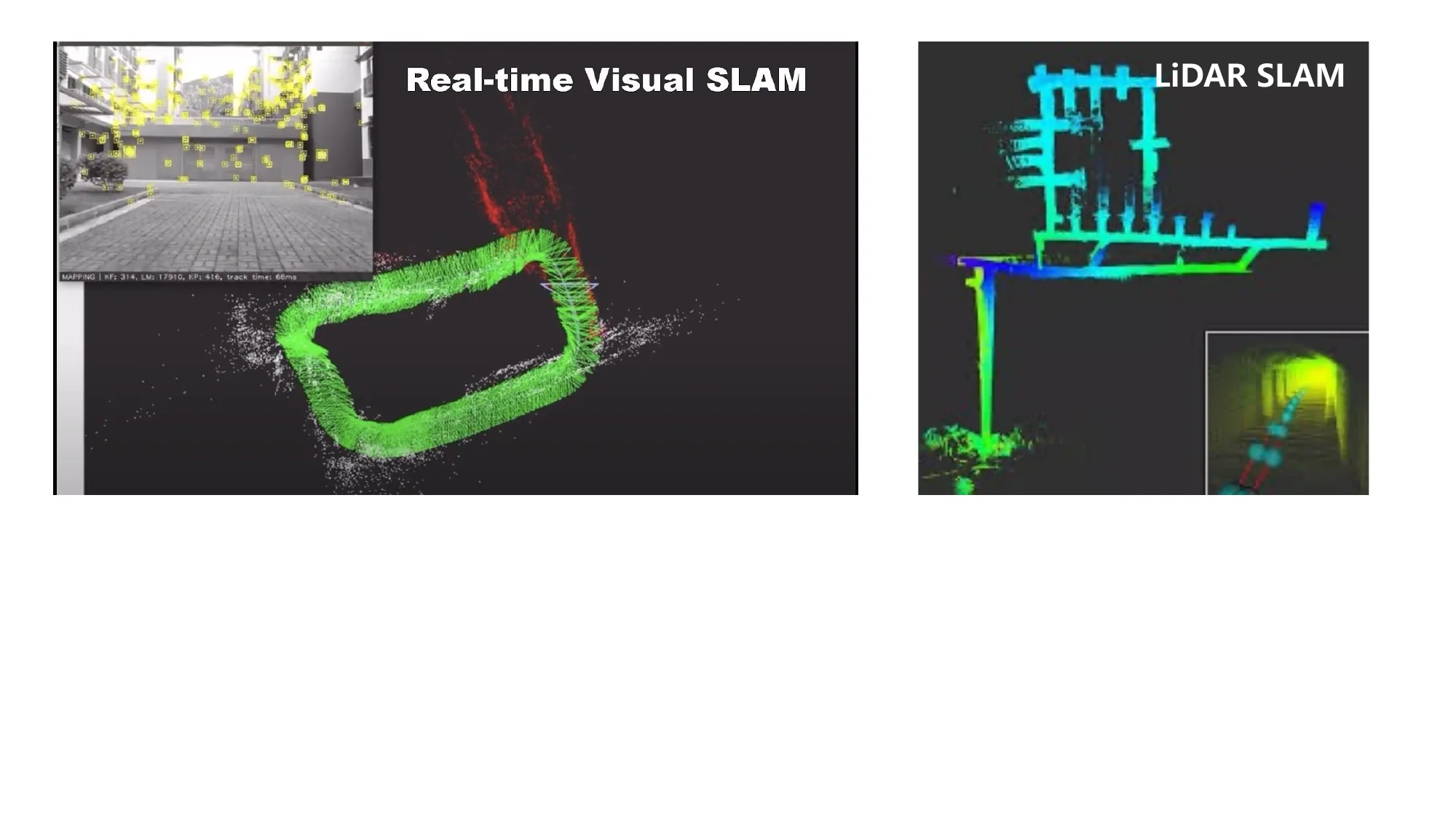
SLAM systems are classified by the exteroceptive sensor and by the density of the map they build. LiDAR SLAM measures range directly with a stable error model; KISS-ICP [928] and KISS-SLAM [929] show that a minimal pipeline delivers robust real-time 3D LiDAR odometry and mapping at city scale. Visual SLAM uses monocular, stereo, or RGB-D cameras, exploiting texture for place recognition, with PTAM [88] and the ORB-SLAM family [91, 736] as the foundational systems. Multi-sensor SLAM tightly fuses cameras with IMUs and/or LiDAR (VINS-Mono, OKVIS, FAST-LIO2), and event-camera SLAM uses asynchronous per-pixel brightness changes for high-speed and high-dynamic-range operation [930]. By map density, sparse keypoint-and-pose-graph systems (ORB-SLAM) sit next to semi-dense direct methods that track image gradients (LSD-SLAM [718], DSO [719]), dense geometric systems that fuse point clouds, meshes, or TSDFs (KinectFusion, ElasticFusion), neural implicit systems (iMAP [923], NICE-SLAM [924], Co-SLAM, NICER-SLAM), and 3DGS systems that render and optimize Gaussians jointly with poses (SplaTAM [925], MonoGS [927], SplatSLAM, MASt3R-SLAM [931]). Read historically, the field moved from feature-based geometry (PTAM, ORB-SLAM) to direct methods (LSD-SLAM, DSO), to tightly coupled multi-sensor systems (OKVIS, VINS-Mono, ORB-SLAM3), to learning-augmented pipelines (DROID-SLAM [95], SuperPoint and SuperGlue matching [539, 541]), to neural implicit and then 3DGS maps, and most recently to 3D geometry foundation models (DUSt3R [122], MASt3R [728], MASt3R-SLAM).
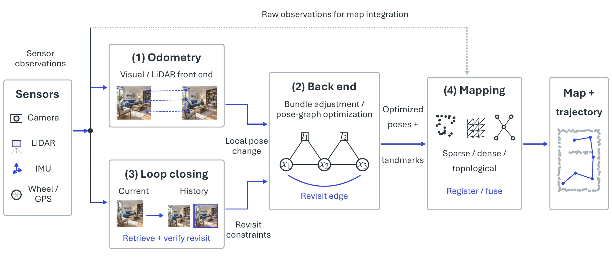
Whatever the sensor or map, a SLAM system runs the four modules of Figure 6.20 in a loop. The front end is visual (or LiDAR) odometry, the incremental motion estimate between consecutive readings treated as a stand-alone task in §6.2.4; because each pose is estimated relative to the last, its errors accumulate as drift. Back-end optimization corrects that drift globally. Modern back ends pose the problem as factor-graph optimization: robot poses and landmarks are nodes, and measurements between them (visual reprojection, IMU pre-integration, GPS, loop-closure relative poses) are factors; solving for all nodes at once yields a consistent trajectory and map, factor graphs absorb heterogeneous sensors naturally, and incremental solvers such as iSAM2 update the estimate in real time, with GTSAM, g2o, and OKVIS as representative libraries. Loop closing supplies the back end with its strongest constraints by recognizing that the agent has returned to a previously visited place, comparing current observations against the history and, on a match, adding a constraint between two temporally distant poses that pulls the accumulated drift of the intervening trajectory back into alignment. Mapping finally places the sensor data in the global frame using the optimized trajectory, in whatever representation the application needs; for neural implicit and 3DGS maps it also minimizes a rendering loss (photometric or perceptual such as LPIPS) between observed images and views rendered from the current map, optimizing geometry, appearance, and poses jointly [925, 931].
| Dataset | Task | Modality | Agent | Scene | Scale | Ground Truth |
| COLD [932] | VSLAM | mono + omni + odom | wheeled | lab | 76 | laser |
| TUM RGB-D [652] | VSLAM | RGB-D | handheld, wheeled | office, work shed | 39 | MoCap |
| KITTI [173] | VSLAM, VO | stereo + laser | car | suburban, highway | 22 | GPS/OXTS |
| ICL-NUIM [933] | VSLAM, VO | RGB-D | synthetic | home, office | 8 | simulator |
| EuRoC [733] | MSLAM | stereo + IMU | drone | work shed | 11 | Vicon MoCap/laser |
| SceneNet [934] | VSLAM | RGB-D | synthetic | home | 15K | simulator |
| TUM VI [935] | MSLAM, VO | stereo + IMU | handheld | campus buildings | 28 | MoCap |
| Bonn RGB-D [936] | VSLAM | RGB-D | handheld | lab | 24 | MoCap |
| InteriorNet [937] | MSLAM | RGB-D + IMU | synthetic | home | 15K | simulator |
| OpenLORIS-Scene [938] | MSLAM | RGB-D stereo + IMU + odom | wheeled | indoor | 22 | MoCap/laser |
| Replica [339] | dense | RGB-D | synthetic | indoor | 18 | simulator |
| ScanNet++ [939] | dense, sem | RGB-D | handheld | indoor | 460 | laser |
| TartanAir [666] | MSLAM, VO | stereo + IMU | synthetic | diverse | 1M+ frames | simulator |
| ETH3D SLAM [940] | VSLAM, VO | stereo + global shutter | handheld | indoor/outdoor | – | LiDAR |
| DSEC [941] | event SLAM | stereo events | car | driving | 53 | LiDAR + GPS |
| CU-Multi [942] | collab. SLAM | RGB-D + IMU | multi-UAV | outdoor | – | MoCap/UWB |
| AirSwarm [943] | collab. SLAM | RGB-D + LiDAR | air-ground | outdoor | – | GPS |
6.3.5.3Datasets and Metrics#
Table 6.24 groups the benchmarks by what they stress. The classical trajectory sets are TUM RGB-D [652] (handheld indoor RGB-D with motion-capture ground truth), KITTI [173] (stereo and LiDAR driving), and the synthetic ICL-NUIM [933] with exact ground truth, while COLD [932] targets topological localization under changing conditions. Visual-inertial systems are tested on EuRoC [733] (micro-aerial vehicle), TUM VI [935], and OpenLORIS-Scene [938], the last built for lifelong SLAM in changing indoor scenes, and Bonn RGB-D [936] isolates dynamic objects. Large synthetic corpora (SceneNet [934], InteriorNet [937], Replica [339], TartanAir [666]) supply photorealistic training and controlled evaluation, with Replica the standard testbed for neural implicit and 3DGS SLAM; ScanNet++ [939] and ETH3D SLAM [940] add laser-scanned geometry for dense reconstruction quality; and DSEC [941], CU-Multi [942], and AirSwarm [943] open the event-camera and multi-agent settings.
Evaluation covers trajectory, map, rendering, and system cost. Trajectory accuracy uses the absolute trajectory error and relative pose error defined in §6.2.4, after aligning the estimated trajectory to the ground truth by a rigid or, for monocular systems, similarity transform; RMSE is the usual summary, with mean, median, and standard deviation also reported. Dense maps are scored by accuracy (mean distance from reconstructed points to the nearest ground-truth point) and completeness (the reverse), summarized by an F-score at a distance threshold, with Chamfer distance common for neural and 3DGS maps. Neural implicit and 3DGS maps add novel-view-synthesis metrics (PSNR, SSIM, LPIPS) on held-out views of the same trajectory. Memory footprint, tracking and mapping frame rates, and end-to-end latency decide embedded deployment [929]. Mature evaluation tools such as EVO2 and the RPG Trajectory Evaluation toolbox3 implement these protocols.
6.3.5.4Challenges#
Deployment exposes SLAM to conditions its assumptions exclude: static scenes, stable illumination, abundant texture, and ample computation. Dynamic objects induce correspondences that drift with their own motion; illumination change, reflective and transparent surfaces, and repetitive texture create perceptual aliasing that confuses data association and place recognition alike; and resource-constrained platforms must run ever heavier front and back ends. Current work answers each directly. Moving features are detected and excluded through semantic segmentation, motion-consistency checks, or learned masks; learned matchers (SuperPoint [539], SuperGlue [541], LoFTR [542]) replace hand-crafted descriptors and tolerate larger viewpoint and illumination changes; neural implicit and 3DGS maps are optimized jointly with poses and yield photorealistic reconstructions usable for inspection, telepresence, and policy learning; and the two-view geometry priors of DUSt3R [122] and MASt3R [728] remove the fragile hand-engineered front end, already enabling real-time dense monocular SLAM at the robustness of MASt3R-SLAM [931].
Two broader shifts follow. Lifelong SLAM aims at months of continuous operation by combining relocalization, map update, and place re-identification against changing environments, and is now an evaluation track of its own; collaborative multi-agent SLAM fuses observations across robots for faster coverage and graceful degradation, increasingly together with event cameras and heterogeneous sensors for high-speed, low-light, and high-dynamic-range conditions. What remains open is concrete: 3DGS maps still do not scale to city-level memory and rendering budgets, learned components carry a sim-to-real gap, and verifying loop closures under strong perceptual aliasing is still the failure that breaks every back end.
- The table is extended from the GitHub repository: https://github.com/ChocoWu/Awesome-Scene-Graph-Generation↩
- https://github.com/MichaelGrupp/evo↩
- https://github.com/uzh-rpg/rpg_trajectory_evaluation↩