11.2.1Introduction#
Geospatial artificial intelligence (GeoAI) applies machine learning to geographic data (satellite and UAV imagery, LiDAR, GNSS traces, and IoT sensor streams) to model and act on processes that unfold over terrain, cities, and the Earth system. It makes the geospatial domain a large-scale deployment target for the perception and scene-understanding capabilities surveyed in Part III: the detection, segmentation, and remote-sensing techniques of Chapter 6 (and the aerial and remote-sensing setting of Section 9.4) are here specialized to Earth-observation data and decision workflows at planetary scale.
11.2.2System Overview#
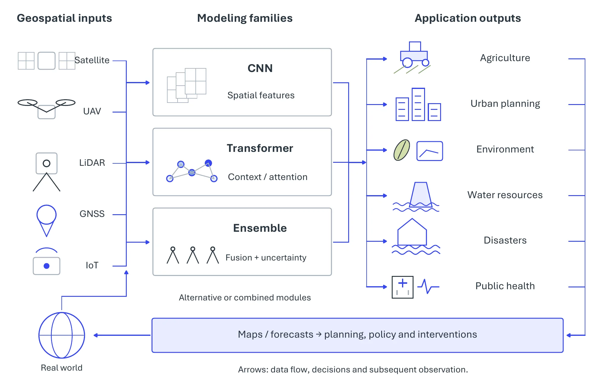
A GeoAI workflow couples heterogeneous geospatial data to models that turn raw observations into spatially explicit decisions (Figure 11.5). Following the application taxonomy of the review by Boutayeb et al. [2698], we treat six domains as pivotal tasks: precision agriculture, the urban built environment, environmental monitoring, water resources, disaster management, and public health. The six share their inputs, largely the free Sentinel, Landsat, and MODIS archives, and until recently they shared a modeling pattern as well: a task-specific supervised network or tree ensemble trained for one region and one target, which the foundation models at the end of the section are beginning to replace. Table 11.2 samples representative data sources, methods, and reported results across the six.
11.2.3Pivotal Task-1: Precision Agriculture#
Precision agriculture tailors irrigation, fertilization, and pest control to the conditions of each field, or each plant, instead of managing a field uniformly. GeoAI supplies the maps and predictions this requires through the complementary mapping, yield-estimation, and irrigation tasks of Figure 11.6.
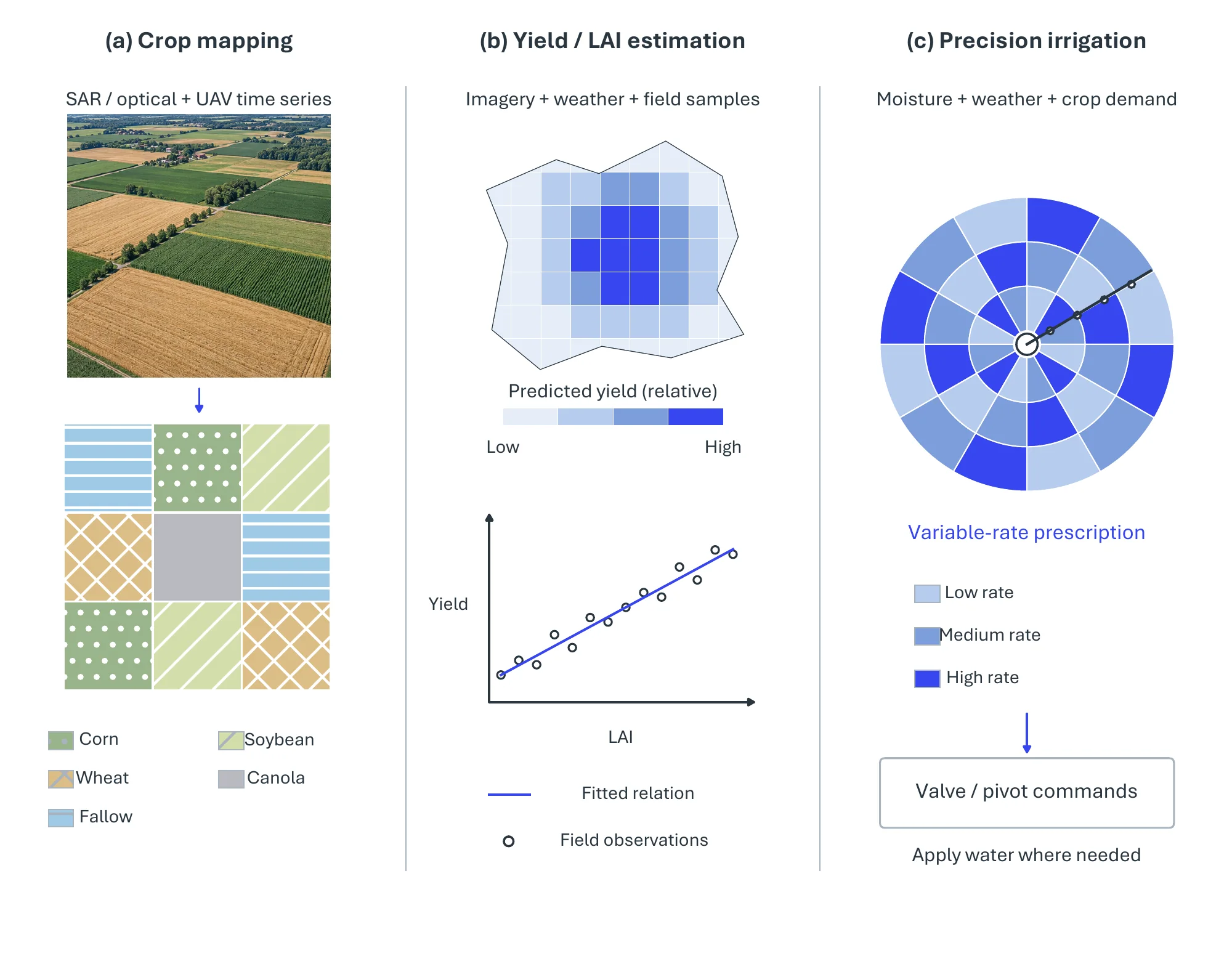
Crops Mapping. Crop mapping turns a time series of satellite or UAV imagery into a per-pixel crop-type label, and the accuracy gains in recent work track the richness of the temporal signal. Han et al. [2699] combine a ResNet feature extractor with cross-attention and spatio-temporal self-attention over Sentinel-1 SAR series, reaching 96% overall accuracy on the Brandenburg benchmark. 3D convolutional networks over Sentinel-2 [2700] and Landsat [2701] series treat time as a third convolution axis, and fusing Sentinel-1 SAR with Sentinel-2 optical data maps rice phenological stages within the season [2702]. Multi-season and SAR–optical inputs consistently beat single-date classification, in part because SAR sees through the cloud that interrupts optical series. At the other end of the resolution range, UAV imagery supports row-level segmentation, where U-Net outperforms LinkNet and PSPNet on sugarcane crop lines [2703].
Yields Prediction. Yield prediction regresses a continuous productivity estimate from the same imagery, and the usual design has two stages: extract a vegetation index or phenotype, then regress. Random forests over Sentinel-2, RTK GPS, and LiDAR variables predict cotton yield [2704], and an ensemble over Landsat-8 NDVI and agro-meteorological data reports R2 0.99 for tea yield on its test set [2705]. UAV imagery earns its extra cost where the target is a fine-grained phenotype: Mask R-CNN extracts wheat-spike phenotypes that feed a yield regressor [2706], and a linear mixed-effect model on fixed-wing UAV multispectral imagery estimates rice leaf-area index and biomass [2707].
Precision Irrigation. Irrigation closes the loop, turning maps and estimates into water-delivery decisions [2708]. One line of work detects irrigation infrastructure at scale, such as center-pivot systems in Sentinel-2 series with Mask R-CNN [2709] or irrigation types in NAIP aerial images with a U-Net and transfer learning [2710]. The other controls water locally: a drone system fuses RGB, thermal-infrared, and GPS data to find the driest zones of a field and sets valve flow with a random forest [2711].
11.2.4Pivotal Task-2: Urban Planning, Logistics, and Transport#
The second task turns GeoAI on the built environment. Figure 11.7 presents five complementary tasks on a shared urban context, from built structure and temporal change to services, transport, and green infrastructure.
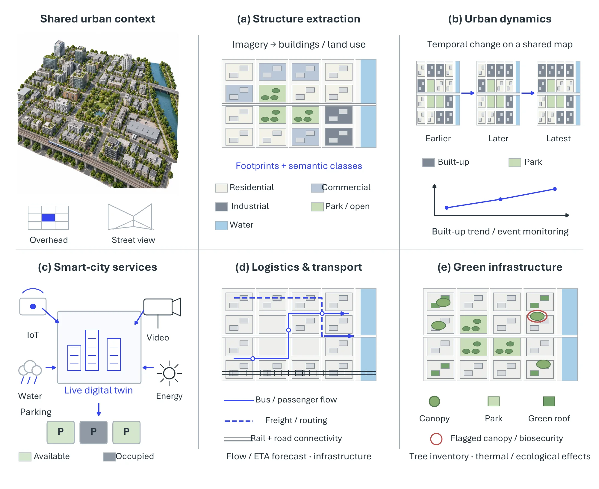
Urban Data Extraction. Land use and built form are classified from overhead and street-level imagery, and fusing the two views resolves ambiguities that neither settles alone. A fine-tuned EfficientNet classifies the 21 land-use classes of the UC Merced set [2712], while a dual-branch network that pairs dilated convolutions on Google Earth imagery with an attention-based multi-view network on Street View detects informal urban villages [2713].
Urban Dynamics. Temporal models capture how urban form changes over time. An LSTM with attention simulates urban densification from land-use rasters of 2000, 2010, and 2020 [2714], and a pix2pix GAN predicts land-use and land-cover change by conditioning Landsat imagery on planning indicators [2715]. A static quantity such as urban solar exposure needs no temporal model; a feed-forward network on building geometry, occupancy, and orientation suffices [2716].
Smart Cities. The service layer turns these representations into live operation: video georeferencing and small-object detection inside an urban digital twin [222], LSTM parking-occupancy prediction served to a mobile application [2717], and detection of commercial signage in Street View imagery to map urban commerce [2718].
Logistics and Transport. Movement through the city splits into two problems with different tools. Flow forecasting is temporal: bus arrival times are predicted from a traffic-density matrix with recurrent and convolutional models [2719], a hybrid GRU–LSTM forecasts traffic from OpenStreetMap and GIS features [2720], IODRNN decomposes its outputs incrementally to remove the lag in GNSS-based forecasts [2721], and itinerary recommendation adds a denoising autoencoder with collaborative learning [2722]. Infrastructure mapping is a segmentation problem: open LiDAR point clouds inventory rockfall-prone road slopes [2723], SegNet on RapidEye imagery updates rural road networks [2724], and U-Net with PointNet++ performs panoptic segmentation of railway environments from multimodal LiDAR [2725].
Green Infrastructure and Bio Security. Vegetation monitoring moves from coverage to function to threat, and each step demands finer spatial and spectral resolution than the last. A semi-supervised DeepLabv3+ maps urban tree cover nationwide from high-resolution satellite imagery [2726]; a Faster R-CNN tree inventory identifies seven canopy species and, through geographically weighted regression, their effect on land-surface temperature [2727]; and biosecurity surveillance of invasive forest pests uses multispectral aerial imagery, where an instance-segmentation model reached an F1-score of 79% against 58% for a tile classifier [2728].
11.2.5Pivotal Task-3: Environmental Monitoring#
The third task observes the Earth system itself, across the three fronts of Figure 11.8.
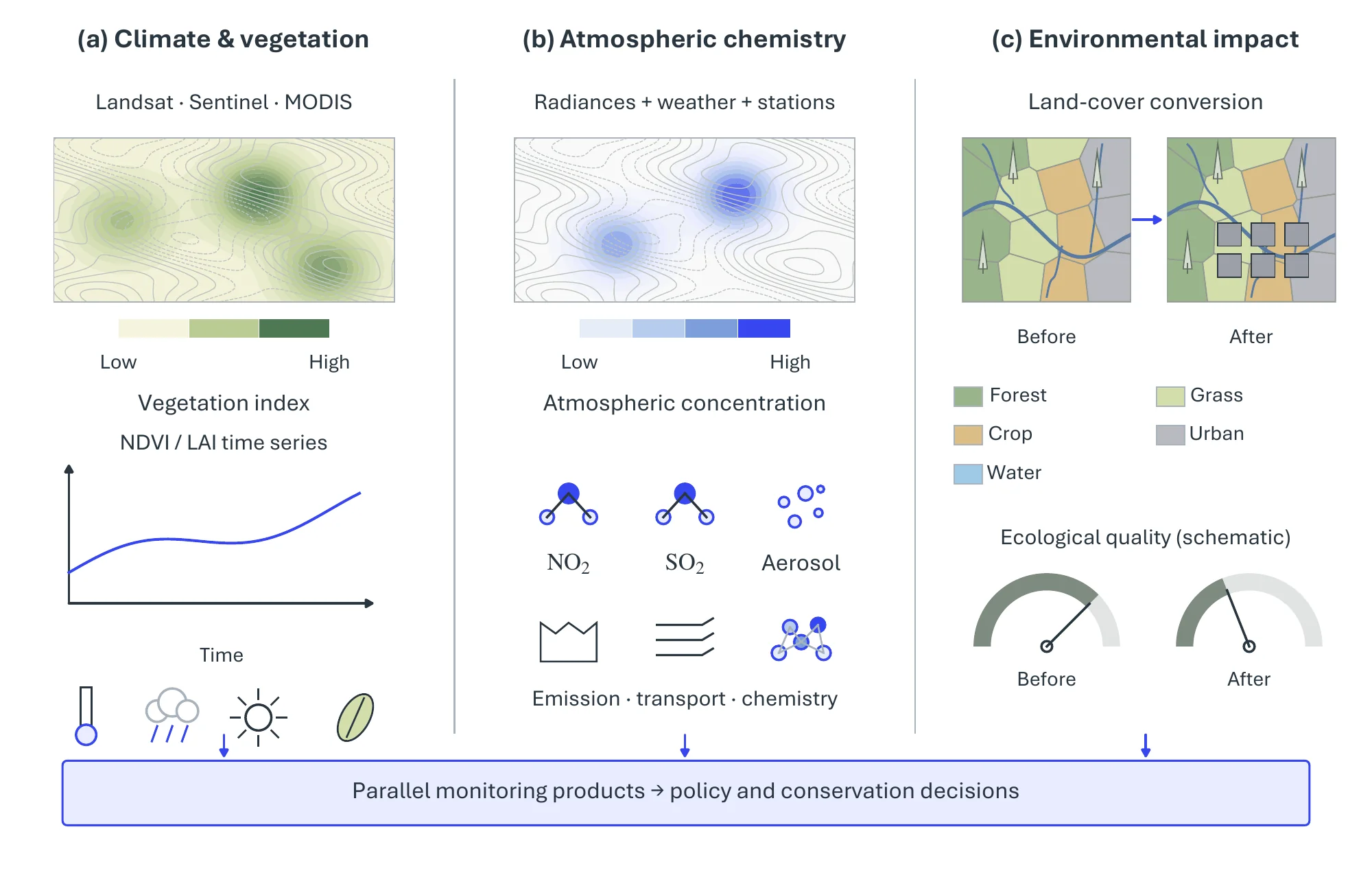
Climate Change. Long-term land-surface change is read mostly through vegetation records spanning decades of Landsat, Sentinel, and MODIS data, and the methods trade spatial detail against record length. Lou et al. [2729] map land use and land cover on Google Earth Engine with a deep network and find rapid greening of the Qinghai–Tibet Plateau from 1988 to 2018. Deep-learning-enhanced spatiotemporal fusion reconstructs long-term NDVI in the Danjiang River Basin [2730], random forests retrieve vegetation phenology from MODIS more accurately than rule-based methods [2731], and a bidirectional LSTM produces the GLASS 250 m leaf-area-index product (version 6) from MODIS reflectance [2732].
Atmospheric Chemistry. Atmospheric composition is retrieved by learning the map from satellite radiances and meteorology to ground-measured concentrations. Nitrogen dioxide is the most studied target, estimated hourly from Sentinel-5P, meteorology, and sensor data with XGBoost [2733] and daily across China with a random forest and K-means clustering over OMI data [9]. A convolutional autoencoder coupled to WRF-Chem models volcanic SO2 dispersion [2734], AQNet fuses Sentinel-2 and Sentinel-5P to predict NO2, O3, and PM10 [2735], an LSTM forecasts five pollutants from ground-station series [2736], and a deep network derives aerosol absorption from the OMI ultraviolet aerosol index, validated against AERONET [2737].
Environmental Impacts. Impact assessment links land-use change to ecological outcomes, and it is judged not only on accuracy but on whether it can name the responsible driver, which is why explainability recurs here. Neural networks on multi-temporal Landsat land-cover maps assess urban ecological quality [2738]; multiscale geographically weighted regression, random forests, and SHAP relate agricultural land to PM2.5 concentrations [2739]; and interpretable ensembles measure the effect of climate change on agricultural land suitability [2740].
11.2.6Pivotal Task-4: Water Resources Management and Precipitation Forecasting#
The fourth task addresses four complementary aspects of water resources in Figure 11.9.
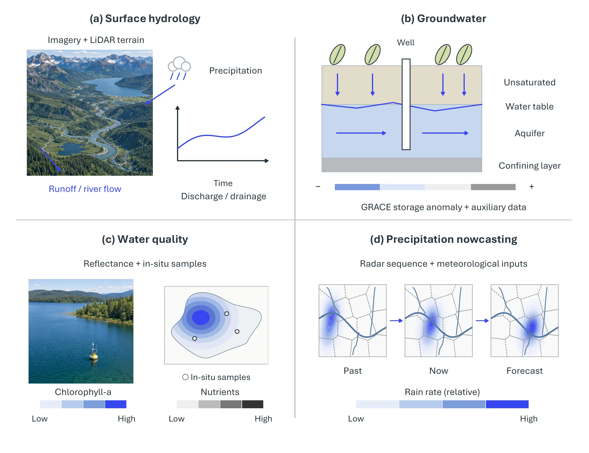
Hydrological Modeling. Convolutional models dominate local surface geometry. Space-time image velocimetry on UAV video estimates river velocity and discharge, validated with LiDAR-derived terrain [2741]; U-Net extracts drainage ditches from LiDAR in low-relief terrain [2742]; quadtree decomposition with multi-scale CNNs extracts coastlines at lower cost than FCN and U-Net baselines [2743]; and a reflectance-transformation CNN maps bathymetry from Landsat and Sentinel-2 imagery [2744]. At basin scale, where streamflow depends on several precipitation products (MODIS, CHIRPS, MSWEP), super-ensembles that weight multiple regressors take over [2745].
Groundwater. No optical sensor sees the water table, so groundwater models work from proxy variables and gravimetry. Static delineation of recharge or shallow-groundwater zones uses tree ensembles and deep networks over hydrogeological and remote-sensing variables [2746, 2747, 2748]. GRACE/GRACE-FO measures total-water-storage changes; isolating groundwater requires auxiliary estimates of other water-storage components. Storage forecasting uses these gravity-derived anomalies, which a CNN–LSTM forecasts with an RMSE of 44.92 mm/month [2749] and which machine-learning regressors downscale to catchment resolution [2750].
Water Quality. Water quality is regressed from spectral reflectance against in-situ samples, and accuracy follows the optical signature of the constituent. Pigments with a clear signature are tractable: fusion of data and classifiers through higher-order SVD estimates chlorophyll-a in Lake Nicaragua [2751], and on UAV multispectral and hyperspectral data of a karst wetland, transformers and gradient boosting predict phycocyanin, dissolved oxygen, and chlorophyll-a, interpreted with SHAP [2752]. Dissolved nutrients remain harder because their optical fingerprint is faint, whether estimated from MODIS with a spatiotemporal deep belief network [2753] or from Landsat-8 with an ANN [2754]. Optical water types themselves can be classified from Sentinel-2 with an SVM [2755].
Precipitation Forecasting. Precipitation nowcasting predicts the next radar frames from the current sequence. HST-AFP fuses radar echoes with weather forecasts through attention [2756], STIN adds humidity, wind, and temperature [2757], and PFST-LSTM adds pseudo-flow estimation to follow echo motion [2758]; at longer range, multi-model ensembles post-process numerical weather prediction [2759].
11.2.7Pivotal Task-5: Disaster Management#
The fifth task covers the disaster lifecycle (hazard or susceptibility mapping, event observation, and damage assessment) for earthquakes, floods, and forest fires, arranged as a grid in Figure 11.10.
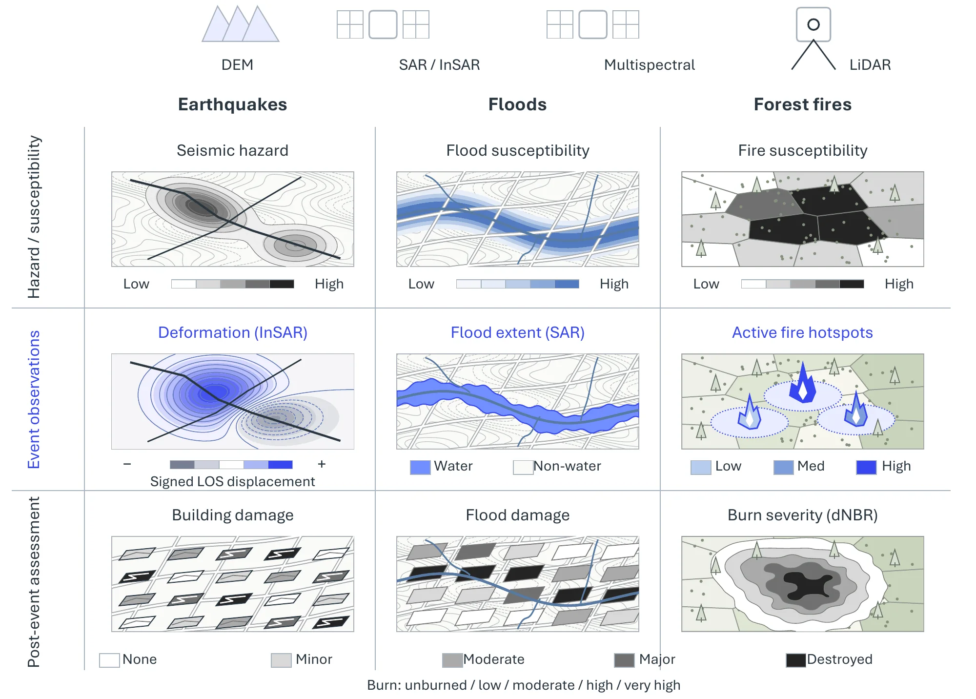
Earthquakes. For earthquakes the lifecycle includes hazard mapping, event-related observation, and damage assessment; these tasks should not be equated with reliable prediction of an exact earthquake. A CNN over elevation, vector, and attribute data maps seismic risk in north-eastern India [2760], and encoder–decoder LSTMs [2761] and neural networks [2762] detect ionospheric anomalies in GNSS total-electron-content data around events such as the 2019 Pakistan earthquake. After the event, LiDAR, orthophotos, and multispectral imagery estimate building vulnerability [2763], and change detection on multi-temporal photogrammetric point clouds classifies structural damage into grades [2764].
Floods. Floods lean on radar. Forecasting fuses meteorological, hydrological, and crowdsourced data, either comparing classical learners under cross-validation [2765] or with a ConvLSTM that learns spatial rainfall patterns and their temporal dynamics jointly [2766]. Inundation mapping falls to SAR segmentation, which sees through cloud, as in an attention-augmented U-Net on dual-polarized Sentinel-1 imagery [2767].
Forest Fires. Fire has the fullest lifecycle. Susceptibility is predicted from drone imagery with temperature and humidity sensing [2768], or from elevation, vegetation indices, and hydrometeorology with a neuro-fuzzy system tuned by an artificial bee colony [2769]. Detection is trained on drone RGB and infrared imagery such as the FLAME 2 dataset [2770] and can be distributed across sites with federated learning [2771]. Burn scars are delineated afterward by a U-Net on PlanetScope RGB and near-infrared imagery, with F1 up to 0.94 [2772].
11.2.8Pivotal Task-6: Healthcare#
The sixth task brings GeoAI to public health, where spatial signals couple disease and environment (Figure 11.11).
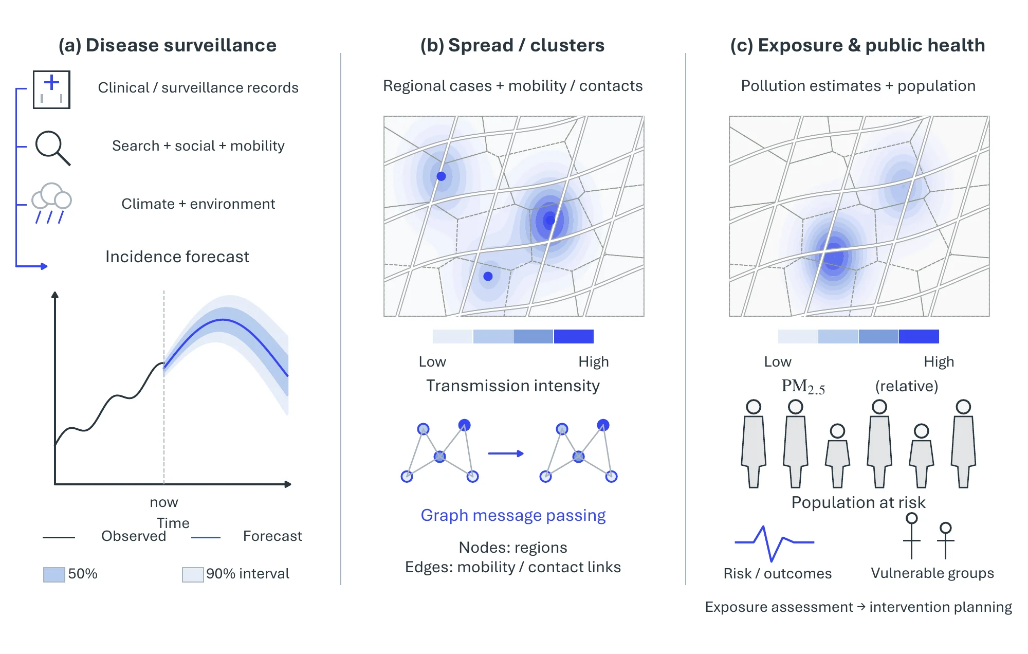
Infectious Diseases and Toxins. Disease surveillance gains most from leading indicators, since search queries and geotagged posts surface an outbreak before clinical reporting does. Influenza forecasting combines CDC surveillance data with Google Flu Trends and climate in a multi-stage LSTM [2773], with geotagged Twitter posts in a neural network tuned by an artificial-tree algorithm [2774], and with search frequencies and health records in a network-based regression that exploits synchrony across U.S. states [2775]; dengue in China is forecast from climate and weekly case counts, with support-vector regression performing best [2776]. FINDER shows the payoff most clearly: it geolocates web-search signals of foodborne illness to restaurants, and the restaurants it flagged were three times more likely to pose food-safety risks than those found by complaint-based inspection [2777].
Pandemics. A pandemic shifts the question to transmission across geography. Geospatial similarity learning predicts respiratory-virus spread in new regions [2778], and spatio-temporal regression tracks COVID-19 in Brazil [2779]. Detection networks catch what an epidemic curve misses: gatherings of people and vehicles in satellite imagery [2780], proximity between re-identified individuals in video [2781], and the drop in PM2.5 during lockdown, measured from MODIS and Sentinel-5P [2782].
Public Health. Chronic exposure links where people are to what they breathe. On the mobility side, mobile health uses wireless devices for clinical and public-health purposes [2783], and the MD2K center turns mobile-sensor streams into markers of smoking, craving, and stress [2784]. On the pollutant side, a geographically weighted gradient-boosting machine [2785] and a neural network over MODIS aerosol optical depth and land-use features [2786] map daily PM2.5 across China and the United States. Exposure assessment is only as sharp as the coarser of the two spatial scales.
| Pivotal task | Representative data source | Representative method | Headline metric |
| Precision agriculture | Sentinel-1 SAR | STMA [2699] | 96% OA (Brandenburg) |
| Precision agriculture | Landsat-8 NDVI + meteorology | Ensemble [2705] | R2 0.99 |
| Urban planning | UC Merced land use | EfficientNet (fine-tuned) [2712] | accuracy |
| Environmental monitoring | Landsat, 1988–2018 | Deep LUCC mapping on GEE [2729] | LUCC accuracy |
| Water resources | GRACE / precipitation | CNN–LSTM [2749] | RMSE 44.92 mm/month |
| Disaster (flood) | Sentinel-1 SAR | Attention U-Net [2767] | precision / recall / F1 |
| Disaster (forest fire) | PlanetScope (RGB+NIR) | U-Net [2772] | F1 0.94 |
| Healthcare | CDC / Google Flu / climate | Multi-stage LSTM [2773] | RMSE / MAPE |
11.2.9Established Tools and Systems#
Cloud geospatial platforms provide planetary-scale storage and analysis next to the data. Google Earth Engine1 offers a petabyte-scale archive of satellite imagery with server-side analysis, Microsoft’s Planetary Computer2 pairs open Earth-observation data with a Python/STAC API, and commercial providers such as Esri ArcGIS3 and Descartes Labs4 deliver hosted GeoAI pipelines for enterprise and government users.
Open-source GIS and ML toolkits carry the modeling layer. QGIS5 is the de facto open desktop GIS, while deep-learning libraries tailored to raster geospatial data, such as TorchGeo6 and Raster Vision7, bridge PyTorch to satellite imagery, and Sentinel Hub8 streamlines on-demand access and processing of Copernicus archives.
Open Earth-observation programmes supply the data foundation: the European Copernicus programme’s Sentinel constellation and NASA/USGS Landsat provide free, calibrated, multi-decadal imagery, complemented by gravimetric (GRACE/GRACE-FO), atmospheric (OMI, Sentinel-5P), and high-resolution commercial (WorldView, PlanetScope) sources that recur throughout the methods above.
11.2.10Toward Geospatial Foundation Models and GeoLLMs#
Almost every method surveyed above is a task-specific supervised model: a CNN, random forest, LSTM, or GAN trained from scratch for one crop, one hazard, or one pollutant. That design is being displaced by the same pretraining-and-transfer paradigm that reshaped the rest of the field (Chapter 7), and the geospatial community has begun building its own foundation models. Masked-autoencoding backbones lead the shift: SatMAE [193] adapts the masked image model to the temporal and multi-spectral structure of satellite imagery, Scale-MAE [2787] makes the pretext task explicitly scale-aware so a single backbone serves the huge ground-sample-distance range Earth observation spans, and Prithvi [2788] packages such a backbone as a generalist model fine-tunable across flood mapping, burn-scar delineation, and crop segmentation. A single pretrained encoder thus stands in for the dozens of bespoke feature extractors that populate the tasks above.
The language side is moving just as fast. RemoteCLIP [2789] aligns remote-sensing imagery with text, giving open-vocabulary retrieval and zero-shot classification without per-class labels; GeoChat [2790] grounds a large vision-language model on overhead imagery so an analyst can query a scene, ask for region-level descriptions, and obtain referring localizations in dialogue; and SegEarth-R1 [2791] pushes further into pixel-level geospatial reasoning, generating segmentation masks from implicit, reasoning-heavy queries rather than fixed class names. These systems inherit the multimodal reasoning and world-model machinery of Part III and specialize it to Earth observation, pointing toward GeoAI workflows driven by natural-language instructions rather than hand-built per-task pipelines.
11.2.11Challenges#
Most of the methods above were trained and tested in one region on one sensor, and that pattern shapes the open problems: whether a model transfers across regions and sensors, how heterogeneous and uneven data are reconciled, whether pipelines run at the scale and latency that operations need, and what new failure modes the geospatial foundation models bring.
Generalization across Regions and Sensors. Few of the studies surveyed test a model outside the region, season, or sensor it was trained on, so their reported accuracies say little about transfer. Crop calendars, building styles, and spectral responses vary from place to place, and a crop map or flood segmenter trained on one country or one satellite can degrade sharply on another. Pretrained backbones such as Prithvi [2788] are motivated by exactly this gap, but systematic cross-region benchmarks remain rare.
Data Heterogeneity and Quality. Geospatial workflows combine imagery, sensor streams, vector layers, and crowdsourced inputs that differ in resolution, revisit time, and reliability, and the volume of these archives makes curation itself demanding [2698]. Open-access data needs quality control before it can serve as training labels. Geospatial data is also strategically sensitive, which raises questions of data sovereignty, and adversarial manipulation of inputs is a threat that none of the methods above addresses.
Scale and Latency. Operational services such as flood mapping during an event, precipitation nowcasting, and traffic forecasting must ingest new acquisitions continuously and update their models as satellites deliver data, which strains pipelines built around one-off training runs. When several models are chained in one workflow, validation and deployment cost grow with each link, pushing systems toward distributed, modular architectures.
Open Problems for Geospatial Foundation Models. The foundation models of the previous subsection bring problems of their own: pretraining that fuses radar, optical, and hyperspectral sensors at very different resolutions; evaluation benchmarks that test geospatial reasoning rather than image-level recognition; and grounding language output in physically consistent, georeferenced coordinates, which dialogue systems such as GeoChat [2790] do not yet guarantee.